Generator forecasting
For 6 solar farms and 3 wind farms over one validation year, the largest gain was from the Met
Office's UKV weather forecast at wind farms, about 0.2 points of capacity at 24 to 54 hours ahead (a
small gain: its interval excludes zero but not the pre-registered 0.15), measured on a research
archive and not the live feed, so it is an upper limit. No input met its pre-registered gain
threshold. Seven of the eight experiments scored forecasts for Tuesday runs from July 2025 to June
2026. The eighth tested a monitor for a lost inverter at the solar farms, and it reliably found only
large, long losses. No experiment in this theme is a candidate for production.
UKV is the Met Office's 2 km weather forecast for the UK. Most experiments start from the ENS weather forecast and ask what one added input does. A negative difference in a score means a better forecast, and a point of capacity is 1% of a farm's effective capacity.
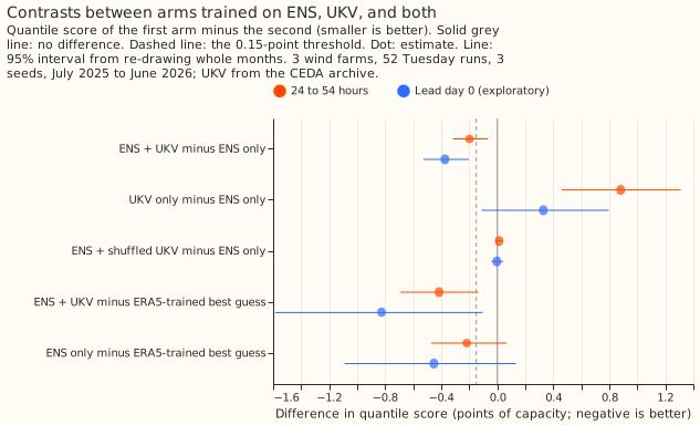
At 24 to 54 hours ahead, adding UKV lowers the wind farms' quantile score by 0.198 points (95% interval -0.316 to -0.069), whereas a shuffled copy of UKV changes it by +0.013 (-0.012 to +0.040). Source: experiment 54. The bars for lead day 0 are exploratory.
Does it work?
A second weather forecast helps wind farms a little and solar farms by an amount the data cannot
resolve. For wind farms, experiment 54
gave UKV's wind to an XGBoost model trained on ENS. The quantile
score fell by 0.198 points, a small gain
because the interval's near end (-0.069) did not reach the pre-registered 0.15. The gain was -0.413
at one farm and +0.018 at another (exploratory). For solar farms, experiment
57 found -0.035 (95% interval -0.119 to
+0.037). That interval excludes gains above 0.12 points and includes the 0.10 that would justify a
new weather feed, so the verdict is inconclusive. Both experiments read UKV from the CEDA research
archive, whose licence is non-commercial and which differs statistically from the live feed, so each
result is a ceiling on what a service could get.
Averaging in two more weather forecasts did not resolve a wind gain. In experiment 52, averaging the quantiles of the best guess with those of the same model fed ICON-EU and the ECMWF high-resolution forecast scored -0.055 (95% interval -0.200 to +0.072) at lead days 1 and 2. The experiment fed runs about half a day older than the ENS run, with uncorrected winds, so it tested a handicapped version of the idea. At days 3 to 6 the blend scored +0.122 (+0.028 to +0.221, worse), because of the spread factor.
Recent power added nothing detectable. In experiment 23, giving the second-stage calibrator (see stages 0, 1a, and 2) the farm's lagged power changed the CRPS by -0.012 for solar (99.58% interval -0.122 to +0.088) and +0.012 for wind (-0.090 to +0.146). The 14-day correction raised the CRPS of the pooled mixture by +0.437 for solar (+0.215 to +0.664) and +0.413 for wind (-0.003 to +0.924), and cut the 5% to 95% band's coverage to 53% to 77%.
A recent-capacity feature and fitted physics gave no gain, and new training inputs gave small ones. These experiments score the CRPS, except experiment 12, which scores the mean absolute error of the 51-member average.
- Recent-capacity feature (experiment 26): solar -0.018 (98.75% interval -0.162 to +0.096), wind +0.013 (-0.054 to +0.101). One solar farm gained 0.235 points and another lost 0.085.
- Fitted physics model in place of the XGBoost stage 1 (experiment 29, 6 solar farms): +0.079 (98.75% interval +0.029 to +0.135), worse. Adding the physics output to the XGBoost columns changed nothing (-0.000, -0.015 to +0.018).
- Satellite sunlight (CAMS) as the training input (experiment 12): -0.140 (99.5% interval -0.277 to -0.044) for solar (6 farms), just short of the pre-registered -0.15. A power-curve base margin for wind gave -0.030 (-0.061 to -0.007), and a training start in 2023 or 2024 moved the error by under 0.3 points.
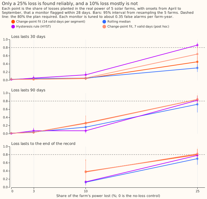
On 5 solar farms with artificial losses added, only a 25% loss was found reliably (0.84 to 0.86
for the best monitor at 90 days, and 0.86 for the hysteresis rule at 30 days), and a 10% loss mostly
was not. Source: experiment 72. The
change-point monitor found 0.84 of 25% losses lasting 90 days and 0.45 of those lasting 30 days,
which breached the pre-registered stop rule of 0.80, so the verdict is refuted. A hysteresis rule
(alarm after 7 valid days at least 10% below normal) found 0.86 of the 25% losses lasting 30 days
but 0.13 or less of 10% losses. The monitor beat neither baseline by an interval that excludes zero:
against the rolling median its difference in detection rate was +0.045 (97.5% interval -0.015 to
+0.090). A farm gives about 3 usable days a week from April to September, and the only real losses
held were one farm's three low months.
Best design so far
No recipe tested here beat the best guess by a pre-registered, resolved margin, so the best guess remains the reference for solar and wind farms. The best guess for farms is a pooled mixture over the 51 ENS members of XGBoost quantile models trained on ERA5, with a spread factor and, for wind, a power-curve base margin. Experiments 23, 26, and 29 used the same mixture without the spread factor as their benchmark.
- Wind, 24 to 54 hours: an XGBoost model trained on ENS and given UKV's wind scored 5.921, against 6.119 for the same model without UKV and 6.337 for the best guess (experiment 54). The contrast with the best guess is exploratory, -0.416 (-0.693 to -0.136), and UKV comes from the research archive.
- Solar, 24 to 54 hours: the ENS-trained model scored 3.140 and the best guess 3.247, a difference of -0.107 (-0.327 to +0.053) that cannot be resolved (experiment 57). Adding UKV scored 3.105.
Candidates for production
None of the eight experiments is a candidate: all are marked not-for-production. The wind
result of experiment 54 would need a matched history of the live UKV feed, and the Open-Meteo
history the experiment found reaches lead day 0 only.
Gotchas and implementation details
- Add a shuffled-input arm beside every arm that adds input columns. The shuffled UKV changed the wind score by +0.013 and the solar score by +0.002, so the gain was not extra columns (experiment 54, experiment 57). In experiment 26 the shuffled solar feature scored 0.023 worse than no feature, so a contrast against the shuffle and one against no feature differ (experiment 26). Re-check: a different model or a larger set of columns.
- Call a UKV result from the CEDA archive a ceiling. The archive is not the live product, so the gain may not reach a service (experiment 54, experiment 57). Re-check: a matched live UKV history.
- Say whether night rows are in a solar score. Experiment 57's pooled score includes night rows, which score near zero, and its daylight-only contrast was -0.074 (-0.259 to +0.079), so check the size on daylight rows as well (experiment 57). Re-check: a pre-registered daylight-only threshold.
- Do not add the mean-error 14-day correction to a farm forecast. Observed power minus the median is positive on average for a right-skewed target even when the quantiles are calibrated, so the correction adds a bias, and coverage fell to 53% to 77%. The post hoc median version scored +0.010 (solar) and -0.064 (wind), with intervals that include zero (experiment 23). Re-check: a daily history, which experiment 23 lacked, because its weekly runs left at most two runs in a window.
- Test recent power in a calibrator trained on pooled members. The calibrator trained on the ENS control member alone scored 0.27 (solar) and 0.31 (wind) points worse than the pooled mixture in the absolute scores (the contrast interval for wind includes zero), so the lag test used a weaker baseline (experiment 23). Re-check: a calibrator trained on pooled members.
- Fit a spread factor under the weights the blend will use. A factor fitted on earlier months blended under other weights made the blend +0.122 worse at days 3 to 6, against +0.005 without it (experiment 52). Re-check: a factor refitted after each weight change.
- Feed other weather products the runs the service would read. Experiment 52 used runs about half a day older than ENS and uncorrected winds, so its null result may understate the products (experiment 52). Re-check: 00 UTC runs of the ENS run's date, with bias-corrected winds.
- Read per-farm contrasts, and treat intervals as covering these farms only. The intervals resample months and not farms. The UKV gain was -0.413 at one wind farm and +0.018 at another, and one solar farm drove the point estimate of experiment 26 (experiment 54, experiment 26). Re-check: more than 6 solar and 3 wind farms.
- Test fitted orientation against a different irradiance-transposition model. A test with the fitted model's own physics showed a tilt bias of +0.11 degrees, and a different sky model showed +6.2 (experiment 29). Re-check: a different fitted physics model.
- Score a monitor on the unmodified record as well as on a placebo. The change-point monitor's false-alarm rate was 0.29 per farm-year on the week-shuffled placebo and 0.54 on the real record, where one farm's winter dip raised 6 of 18 alarms (experiment 72). Re-check: another year of record.
What we have not settled
- Whether the live UKV feed gives wind farms the gain the research archive did, which needs a matched live history at lead days 1 and 2.
- Whether solar farms gain from a source of a different kind, such as a satellite-based nowcast, since UKV here added little, and a second global ensemble added under 1% to the sunshine forecast at five Primary substations (experiment 50, as experiment 57 reports it).
- Whether a wind feature of 75th-percentile power over wind speed cubed helps. It scored -0.061 (-0.107 to -0.025) in experiment 26's contrast C5, one of its 12 contrasts and outside the 4 that decide the verdict.
- Whether CAMS-trained solar models hold their -0.140 on more than 6 farms or a second year.
- Whether a loss of 10% or less at a solar farm can be found from outage notices or trip logs, which need labelled events.
- Whether ENS-trained wind models beat the ERA5-trained best guess at 24 to 54 hours: -0.218 (-0.472 to +0.069) in experiment 54.
The Experiments page lists every experiment in this theme, and the Research plan lists what is planned next.