Does a differentiable physics stage 1 beat the XGBoost stage 1 for solar farms?
We asked whether a solar forecasting model built from the physics of a solar panel, with its parameters fitted by gradient descent, beats an XGBoost model for solar farms. We fitted the physics model and combinations of it with XGBoost for 6 solar farms, and compared their forecast accuracy. No combination beat XGBoost, and the physics model alone was worse by 0.079 points of capacity.
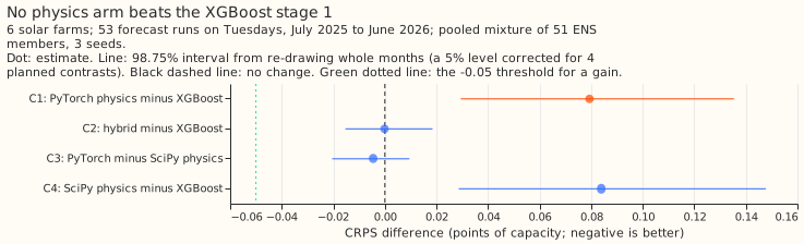
Verdict: refuted. No physics arm lowered the continuous ranked probability score (CRPS) of the XGBoost stage 1, and the PyTorch physics stage 1 alone scored 0.079 points of capacity worse (98.75% interval +0.029 to +0.135).
This page is proposal P31 in the research plan. ENS is the ECMWF ensemble, ERA5 is the ECMWF reanalysis, and CAMS is the Copernicus Atmosphere Monitoring Service's satellite irradiance estimate. Farms appear only under anonymous labels A to F.
Survey of the earlier PV fits (step 1)
The best fitted PV model in the earlier studies was a five-parameter physical model with free
orientation, and it still trailed XGBoost. The beam-diffuse
study fitted tilt, azimuth, capacity, an inverter limit, and a
temperature coefficient per farm with a Powell optimiser. On CAMS irradiance it scored 6.28% of P99
output against 5.24% for XGBoost, and an XGBoost calibration that saw the weather closed most of the
gap. The solar BMU study found that a free orientation
held out better than a fixed or tracking plant, and recovered simulated plants' tilt with a +9.6
degree bias. Chosen: the SciPy free-orientation fit (studies.pv_fit) as the scipy arm, and
for the PyTorch PV model the ideas the differentiable-physics page proposes: priors on tilt,
azimuth,
DC capacity, and the AC-to-DC ratio, a smooth clip, and a posterior for intervals. The SciPy model
is the best fit in the two earlier studies we read, so it is the comparison for the new PyTorch PV
model.
Results
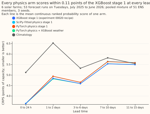
- Absolute CRPS, all leads (points of capacity): XGBoost stage 1 5.026 (95% interval 3.729 to 6.494), hybrid 5.026, PyTorch physics 5.105, SciPy physics 5.110, climatology 5.629. Seed spread is at most 0.001.
- C1 PyTorch physics minus XGBoost: +0.079 (+0.029 to +0.135). C2 hybrid minus XGBoost: -0.000 (-0.015 to +0.018). C3 PyTorch minus SciPy: -0.005 (-0.020 to +0.010). C4 SciPy minus XGBoost: +0.084 (+0.029 to +0.148). The rule refutes the hypothesis when the lower bounds of C1 and C2 are both above -0.05, and they are (+0.029 and -0.015).
- Stage 1 alone: the member-average physics power has a mean absolute error of 7.44 points (SciPy) and 7.53 (PyTorch), against 7.64 for experiment 00012's XGBoost stage 1a on the same rows. This comparison is descriptive: experiment 00012's CAMS-trained arm scored 7.50, level with the PyTorch physics, and the rows may differ. The cause of the CRPS gap was not isolated; a possible cause is the spread that the XGBoost layer builds from one physics column.
- Coverage of the 5% to 95% band: SciPy 96.6%, PyTorch 96.5%, hybrid 94.8%, XGBoost 94.7%.
- Fitted parameters: the table below gives every fitted parameter. Five of the six PyTorch tilts fall in the beam-diffuse study's 14 to 27 degrees, and farm E is higher; every azimuth is within 5 degrees of south, as in that study. SciPy values are within 3 degrees of tilt of the PyTorch values for five farms, and within 0.07 of capacity.
Fitted parameters, by anonymous farm label. The metadata holds no tilt or azimuth, so both are inferred. The fit works in fractions of each farm's effective capacity, the 99th percentile of its absolute power over the history, which is not the farm's registered capacity. The MW values are those fractions times the effective capacity in MW. Intervals are 90% posterior intervals from the PyTorch fit, and the SciPy fit gives point values only.
| Farm | Effective capacity (MW) | PyTorch tilt (degrees) | PyTorch azimuth (degrees) | PyTorch DC capacity (MW) | PyTorch AC capacity (MW) | PyTorch DC:AC ratio | SciPy tilt (degrees) | SciPy DC (MW) | SciPy AC (MW) |
|---|---|---|---|---|---|---|---|---|---|
| A | 6.0 | 25.2 (23.0 to 27.2) | 180.2 (177.6 to 182.9) | 6.8 (6.7 to 6.9) | 5.9 (5.6 to 6.1) | 1.15 (1.11 to 1.20) | 26.5 | 6.6 | 5.8 |
| B | 7.8 | 20.9 (19.3 to 22.4) | 180.1 (177.5 to 182.6) | 8.9 (8.8 to 9.0) | 7.6 (7.3 to 7.9) | 1.17 (1.13 to 1.22) | 22.2 | 8.7 | 7.5 |
| C | 7.9 | 18.0 (16.6 to 19.4) | 179.3 (176.3 to 181.9) | 9.4 (9.3 to 9.5) | 7.7 (7.5 to 7.9) | 1.22 (1.18 to 1.25) | 19.1 | 9.2 | 7.6 |
| D | 1.2 | 24.2 (21.2 to 27.3) | 178.7 (175.3 to 182.0) | 1.4 (1.4 to 1.5) | 1.0 (1.0 to 1.1) | 1.42 (1.36 to 1.47) | 26.7 | 1.4 | 1.0 |
| E | 17.6 | 35.0 (26.1 to 42.8) | 180.3 (175.1 to 185.9) | 16.4 (15.8 to 17.1) | 14.7 (13.5 to 15.6) | 1.12 (1.06 to 1.21) | 34.9 | 16.1 | 15.8 |
| F | 6.0 | 20.7 (19.3 to 22.1) | 179.9 (177.2 to 182.3) | 7.4 (7.3 to 7.4) | 5.9 (5.7 to 6.0) | 1.26 (1.23 to 1.29) | 22.0 | 7.2 | 5.7 |
Comparison with NGED's Embedded Capacity Register (ECR), by anonymous farm label. We matched each farm to ECR rows only where the farm's name equals the ECR's customer name or customer site exactly (ignoring case and punctuation) and the licence area agrees, with no fuzzy matching. The PyTorch DC capacity is compared with the ECR's already connected registered capacity, and the PyTorch AC capacity with the ECR's maximum export capacity.
| Farm | ECR match | ECR status | ECR registered capacity (MW) | ECR maximum export capacity (MW) | Fitted DC over registered | Fitted AC over export |
|---|---|---|---|---|---|---|
| A | no match | |||||
| B | no match | |||||
| C | no match | |||||
| D | no match | |||||
| E | one row | Connected | 18.7 | 17.9 | 0.88 (0.84 to 0.91) | 0.82 (0.76 to 0.87) |
| F | no match |
Only farm E matched, and its fitted capacities are 12% (DC) and 18% (AC) below the ECR. The fitted DC capacity interval (15.8 to 17.1 MW) excludes the registered 18.7 MW, so the interval does not cover the register. Farm E's effective capacity of 17.6 MW is about 98% of the export capacity, which means the metered peaks sit at the export limit. The fitted AC capacity of 14.7 MW is below that observed peak, so the physics model does not reach the metered peaks, which may explain the shortfall; we did not test this. The effective capacity therefore tracks the ECR export capacity and the fitted values do not. The other five farms are named differently in the ECR from the metadata, so their comparison is empty.
Synthetic test (result)
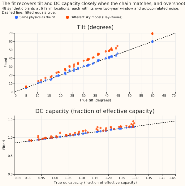
- Same physics, 36 on-prior plants: tilt bias +0.11 degrees, azimuth -0.02, DC capacity -0.005, and 90% interval coverage of 92%, 100%, 97%. AC limit coverage 86%, DC:AC ratio 89%. This passes the pre-registered coverage rule (at least 80% for DC, AC, and ratio). Twelve off-prior plants (tilt 5 or 60, azimuth 110 or 250) give tilt bias -0.05 and azimuth bias +0.76 degrees.
- Different chain (Hay-Davies sky): tilt bias +6.2 degrees (+3.8 off-prior), 0% tilt coverage, DC capacity bias +0.041 (8% coverage). The intervals reflect noise and not the mismatch of the physics, so they are overconfident under mismatch.
Failures and limits
- 6 farms, one validation year: gains under about 0.1 points cannot be resolved.
- The synthetic noise is additive and homoscedastic, and the different-chain version changes only the sky-diffuse term. The likelihood is a tempered pseudo-Huber and not a normalised likelihood, so posterior widths are approximate.
- No post hoc tweak was run.
- Predictions versus outcomes: C1 was predicted between +0.1 and +0.5 and came out at +0.079,
just below that range. The hybrid within 0.05 of
baseand the different-chain tilt bias under 10 degrees were both met.
Lessons
- Fitted PV physics is a competitive point forecast and a poor replacement for the XGBoost stage 1 in the quantile pipeline. The XGBoost stage 1 sees ENS irradiance, temperature, and cloud-related columns that the physics model does not.
- The orientation and capacity the PyTorch PV model recovers are plausible and agree with the SciPy fit, so the physics is useful for interpretation and for checking a farm's metadata.
Arms
| Arm | Stage 1 | Stage 2 |
|---|---|---|
base |
00020's XGBoost quantile stage 1 on nine ERA5 weather columns | Pooled mixture over 51 members |
scipy |
Fitted PV model from studies.pv_fit (free orientation, SciPy), run on each member's shortwave |
One XGBoost quantile model per farm on the physics power only, members pooled |
torch |
New PyTorch physics model with priors | One XGBoost quantile model per farm on the physics power only, members pooled |
torch_hybrid |
The torch output |
XGBoost quantile model on the physics power plus the nine weather columns |
climatology |
None | Month-by-half-hour climatology |
Fitting. Physics parameters are fitted once per farm to metered power at rows before
2025-06-17, using CAMS shortwave and ERA5 temperature (CAMS exists for only part of the history,
so rows without it are left out). Prior means and widths come from general knowledge about Great
Britain's plants (studies.pv_fit.LOOSE_PRIORS), not from any fit to these farms. The stage 2 layer
trains on physics power driven by ERA5
shortwave (base's weather source), and is applied to ENS members' shortwave. CAMS arrives about 1
day late and ERA5 about 5 days, but neither is read at forecast time (the arms read ENS shortwave
and ENS temperature), because no arm uses a lag.
PyTorch PV model. The AC limit is the DC capacity times the AC-to-DC ratio (below 1). The model applies an Erbs split of global into beam and diffuse, isotropic-sky transposition onto a plane of fitted tilt and azimuth, a temperature derate, a DC capacity (a multiple of effective capacity), and a soft clip at DC capacity over an AC-to-DC ratio. Parameters have normal priors and a mean-field normal posterior fitted by stochastic variational inference (Adam, GPU).
Synthetic test (step 2)
Thirty-six synthetic plants (6 farm coordinates times 6 parameter draws: tilt 10 to 45 degrees,
azimuth 150 to 210 degrees, DC capacity 0.9 to 1.3, AC-to-DC ratio 0.7 to 1.0) are driven by the
real training irradiance and temperature of their coordinates, each with its own random two-year
window and noise draw (autocorrelated noise, 4% of capacity). Two versions run: same physics
(the PyTorch PV model's own chain), and different chain (the Hay-Davies sky from pvlib in
place of the isotropic sky, so the fit cannot reproduce the data exactly). The write-up gives each
parameter's bias and 90% interval coverage, each plant's clipping share, and the fit's mean absolute
error.
Checks before the contrasts are read
- Leakage. Every fit, including the physics parameters, stops before 2025-06-17. A reviewer reads the code for this.
- No calendar columns in any stage 2 layer; the hybrid's nine columns are
base's. - Reproduction.
baseis read from 00020's stored predictions, and its solar CRPS is checked against 5.05 within 0.05.
Size
Complex, because the experiment adds a new method and admits more than one defensible design.
- What gets stored: private predictions only.
- Production serving path: not touched.
- Degradation rule: not touched.
- More than one defensible design: yes (the transposition model, the prior widths, whether the stage 2 layer reads the weather).
- Code whose callers cannot be named without searching: no; the code copies experiment 00020's
patterns and calls
studies.pv_physics,studies.pv_fit, andstudies.experiment_store.
Which earlier advice this plan follows
- Followed:
base's absolute score and a climatology row sit beside every contrast (00012, 00020); no calendar columns (skill rule); a contrast is read against a threshold set by the cost of the change (00020). - Departs from: 00012's advice to test CAMS-trained solar on more farms; this experiment keeps the 6 farms, so it cannot resolve gains under about 0.1 points.
Resolution limit
6 farms in one region and one validation year resolve gains of roughly 0.1 points of capacity.