Solar disaggregation

At the 5 Primary substations with a clean solar-capacity estimate, giving the XGBoost demand forecast a forecast of the output of the solar panels behind the substation lowered its daylight April-to-September error by 0.15 points of capacity in one validation year; against a reference that also starts from zero the gain is 0.08 (post hoc, 95% interval -0.11 to -0.05).

A Primary substation's meter reads demand minus the output of the solar panels connected below it, and NGED does not meter those panels. A least-squares fit of calendar-and-temperature demand minus a solar capacity times a satellite-based sunshine shape recovers most of the solar capacity of solar-farm output that we added to real series. The forecast gain depends on the sunshine forecast: a term built from the true sunshine lowers the error by about a fifth, and a term built from the ECMWF ensemble forecast gains little beyond 2 days ahead.

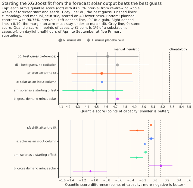
Arm am (the forecast solar output, given to XGBoost as a base margin) scores 4.467 against 4.620 for d0, the best guess of experiment 33, and every arm scores better than its own placebo twin (the same arm given the sunshine of another date). Source: experiment 64. Scores are quantile scores in points of capacity; lower is better. The rows are daylight half-hours of April to September at the 5 Primaries (D9, D10, D11, D14, and D16), from July to September 2025 and April to June 2026.

Does it work?

A simple fit finds most of the solar capacity that we inject, and the capacity is close to unbiased on pure solar output. On the 8 Primaries metered in both directions, the daily fit recovers 0.854 (95% interval 0.815 to 0.866) of the capacity of real solar-farm output added to the demand, and the half-hourly fit 0.773 (0.740 to 0.818). Six of the 8 pass four checks on their real series: placebo sky, season, cloud term, and day type (experiment 39). A misfit test gives a median capacity of 0.992 of the truth on pure solar output (0.951 to 1.032), but detects a load that follows the day's mean cloud in only 0.35 of trials (experiment 40).

An explicit solar term lowers the error of the XGBoost forecast, and the sunshine forecast limits the gain. Built from the true sunshine, the term lowers the score of d1l (d0 without its radiation inputs) by 0.966 (97.5% interval -1.431 to -0.595). Built from ENS sunshine with a coefficient fixed at 1, it lowers it by 0.056 (-0.191 to +0.064), short of the 0.35-point gain the plan required (experiment 46, refuted). With a weight fitted per series, forecast-horizon band, and season, and the term given as a base margin, the score of d0 falls by 0.152 (98.75% interval -0.199 to -0.111), and by 0.272 (-0.420 to -0.145) under 48 hours. With monthly refits the explicit term gains 0.149 (99.17% interval -0.201 to -0.104) and three same-time sunshine analogues gain 0.095 (-0.185 to -0.007); the two are not separated, and the verdict is inconclusive (experiment 74).

Beyond 10 days all of the gain, and over all leads about half of it, is XGBoost starting from zero. Beyond 10 days the fitted weight is zero, yet a refit with a base margin of zero and no solar term scores 0.102 below d1l and am 0.098 below d1l (both uncorrected, 95% intervals; experiment 76). Over all leads am is 0.152 below d0 and 0.082 below a d0 that starts from zero (-0.113 to -0.052; post hoc, 95%; experiment 78). Whether a zero start matters in production-style forecasts is not settled: see the gotcha below.

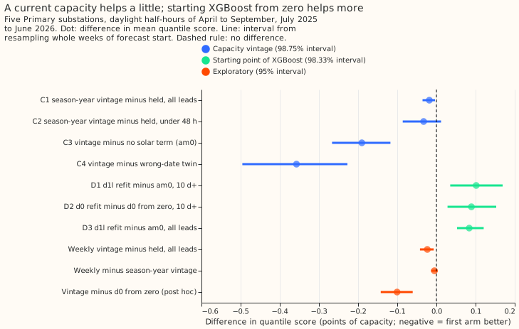
The starting-point read in this figure is for am_sy (am with a capacity re-estimated each season-year), which is 0.100 below d0 started from zero, not the 0.082 of am. Source: experiment 78.

Neither the panel shape nor a fresher capacity is where the next gain lies. A fitted blend of east-, south-, and west-facing shapes changed the score of am by -0.001 (98.33% interval -0.018 to +0.014) (experiment 77, refuted). A capacity re-estimated before every forecast run lowered it by 0.018 (98.75% interval -0.036 to -0.004), under the 0.05 threshold (experiment 78, small gain).

A weekly capacity series, the panel mix, and a loss monitor were not shown to work. A weekly capacity fit that penalises falls more than rises recovered none of a 30% fall and gave 0.66 false steps per Primary-year, against a limit of 0.5 (experiment 45, refuted). The east-south-west shares were not identified: the median share error with noise was 0.200 against a limit of 0.15, although the blend predicted held-out blocks 1.3% better than all-south panels (98.75% interval -2.4% to -0.5%; experiment 73, partly supported). A change-point monitor of a solar farm's daily output found 0.84 of 25% losses lasting 90 days and 0.45 of those lasting 30 days (experiment 72, refuted).

At the 8 Primaries metered only in MVA, the real readings showed almost no reverse flow, so the fit could not be tested on them. In the injection test at the 8 MW-metered Primaries, with the sign of the readings hidden, the unfolding fit's median capacity error was 0.092 against 0.290 for a naive fit, and its balanced accuracy for the direction of flow 0.78 to 0.81, below the 0.80 the rule needed. On the real MVA-only Primaries the fit found no reverse flow at 7 of 8; at the eighth the flow is negative on 75% to 87% of daylight half-hours from 2021, and signed power is needed to check it (experiment 79, partly supported).

The data could not tell us whether the gain holds in a second year, at Primaries without a clean capacity estimate, or on rows outside April to September. The weights of experiment 64 rest on one July-to-September period.

Best design so far

The best of the recipes tested in this theme gives XGBoost a solar offset built from a solar capacity per season-year and a calibrated ENS sunshine anomaly. The steps are:

1. Fit one solar capacity per Primary per season-year, by least squares, and refresh it once per season-year (experiment 39, experiment 45, experiment 78).
2. Multiply the capacity by the calibrated ENS sunshine anomaly: how much sunnier or cloudier the day is than average for that month and half-hour, rescaled by a slope fitted on the training window. The weight is fitted per series, forecast-horizon band, and season, and is zero from 10 days (experiment 64).
3. Give the product to XGBoost as a base margin, not as an input column or a shift after the fit: am beats the input-column arm by 0.093 (95% interval 0.057 to 0.129, exploratory; experiment 64).
4. Use an all-south panel shape (experiment 77).

Candidates for production

Experiments 64 and 78 are candidate.

• The solar offset (experiment 64). Production would need a capacity table, a table of weights, the ENS calibration slopes at predict time, and a base margin set on each prediction matrix; the write-up says the live service cannot supply these as built.
• Refresh the capacity table once per season-year (experiment 78). A weekly vintage differs from the season-year vintage by -0.005 (95% interval -0.013 to +0.003, exploratory).
• A zero start is untested in production-style forecasts, so it is not yet a candidate. Experiment 78 advised testing it; experiment 80 could not tell the two starts apart.
• The offset's gain inside the full forecast is 0.114 on the rows it can touch. In BG2 (a blend of XGBoost forecasts, with the offset at 5 of 16 Primaries) the offset lowers the score by 0.114 (0.075 to 0.164) on April-to-September daylight rows of the 5 offset Primaries, and by 0.010 (0.000 to 0.019) over all rows of the 16 Primaries, because only 8.5% of those rows can carry an offset. The gate was chosen on the same validation year (experiment 87).

Gotchas and implementation details

Score a zero-start twin before crediting an input. XGBoost's estimated starting prediction (its base score) raised the score of d0 by 0.071 over all leads (zero start minus estimated start -0.071, -0.099 to -0.047), and the gain of am where its weight is zero is reproduced by a refit with a zero margin and no solar term (experiment 76, experiment 78). Experiment 80 (inconclusive) could not tell a zero start from the default at the 16 Primaries refitted weekly (-0.017, 98.75% interval -0.072 to +0.054, which does not exclude -0.07). Re-check: the zero-start twin of whichever recipe, correction, and number of boosting rounds you use (experiment 80).

Give every solar-term arm a placebo twin. The twin of am scores 0.300 worse (0.198 to 0.407), so the gain comes from the timing of the sunshine. Shift the twin cyclically and do not permute it at random: a random permutation paired runs that forecast the same valid time, so the permuted anomaly stayed correlated with the real one (experiment 64, experiment 77). Re-check: a different sunshine source. These experiments ran no shuffled-capacity control.

Report each contrast with and without the 14-day correction. The correction carried the base margin's effect from shorter leads into leads beyond 10 days: am minus am0 was -0.035 corrected (98.33% interval -0.074 to +0.003) and +0.004 uncorrected (95% interval -0.012 to +0.021) (experiment 76). Re-check: a forecast with a different correction window.

Score a solar term on daylight April-to-September rows that have both a CAMS shape and an observed power, and name the row set. Experiments 46, 64, 74, 77, and 78 share 68,903 rows per seed. Experiment 87's headline scored all rows of all 16 Primaries, so its 0.010 cannot be compared with 0.15; on the matching gated rows it found 0.114 (experiment 46, experiment 87). Re-check: a study that scores winter or night rows. CAMS is the Copernicus satellite sunshine estimate (glossary).

Check a contrast's sign in each valid month before reading the pooled interval. The ENS solar term lowered the score of d1l in April, May, and September (-0.204, -0.232, -0.262) and raised it in June, July, and August (+0.117, +0.183, +0.024) under a pooled interval of -0.191 to +0.064 (experiment 46). Re-check: a validation period longer than 6 valid months.

Use one capacity per season-year, which runs from September to August in these experiments. The differentiable-physics code runs it from July to June. The latest week of a real-time weekly estimate had 3.63 times the path error of the same week in the final fit, and no penalty pair met the limits (experiment 45). Re-check: a penalty set per Primary, which experiment 45 did not test.

Do not treat a fitted capacity as a measurement. The fit can absorb cloud-driven demand, and the misfit test misses a load that follows the day's mean cloud. Run the placebo-sky, season, cloud-term, and day-type checks on the real series, and inject more than one farm: the ratios of Solar farm E left the capacity at 0.825 of the truth (experiment 39, experiment 40). Re-check: an independent register of installed solar.

Do not publish the fitted orientation shares. They changed by a median 0.24 between consecutive season-years, and the 1.3% fit gain did not reach the forecast (-0.001; experiment 73, experiment 77). Re-check: shares fitted on a longer record, or a known answer with the real noise that they recover to within 0.15.

Do not fit a signed model to an MVA-only series. The magnitude folds reverse flow into positive power, and in the injection test at the 8 MW Primaries the naive fit's capacity error was 0.29 to 1.00 (experiment 79). Re-check: a few weeks of signed power at the Primary in question.

Read coverage as well as the score. The ENS solar term moved the share of sunny-row actuals below the 0.05 quantile from 0.151 to 0.045, though the score barely changed (experiment 46). Re-check: coverage on sunny and cloudy rows for any new solar term.

What we have not settled

• Whether the gain holds in a second validation year and beyond the 5 Primaries with a clean capacity estimate.
• Whether a better sunshine forecast closes the gap to the true-sunshine oracle. The NOAA GEFS ensemble was refuted as a replacement for ENS. The Met Office UKV blended with ENS gave a small gain in squared error of the sunshine-anomaly forecast (not of demand), and the UKV archive used has a non-commercial licence (experiment 50, experiment 53).
• Why the true-sunshine term loses at sunny summer middays: the coefficient of 1 is too large, and the cause is not identified (experiment 51).
• Whether a solar term helps a joint demand fit (experiment 63, experiment 104).

The Research plan lists the proposed next experiments.