No weather product we tested reliably beat ECMWF's ensemble mean at 6 solar and 3 wind farms, and a blend lowered the wind error at a lead a live service could use

At 6 solar farms and 3 wind farms in Lincolnshire, none of the weather products we tested beat the mean of the European Centre for Medium-Range Weather Forecasts (ECMWF) ensemble forecast (ENS, the mean of 51 ensemble members) at a matched lead, and a blend of products lowered the wind error at a lead a live service could use. Each comparison gives one product's weather forecast to an XGBoost model (a gradient-boosted tree model) and scores the power forecast that the XGBoost model makes as a mean absolute error, in percentage points of the generator's capacity (its 99th percentile of metered output). A forecast's lead is the time from the start of the run that made it to the hour it forecasts.

A difference is the first product's error minus the second's, so a positive difference means the first product forecasts worse. Each bracketed pair is a 95% interval. A matched lead needs explaining, because Open-Meteo's archive of past forecasts cannot give the two products the same lead. The study therefore scores ENS at two leads, one shorter and one at least as long as the other product's lead. If a product beats ENS at ENS's shorter lead, the product wins even though ENS had the advantage. If ENS beats a product at ENS's longer lead, ENS wins even though the product had an equal or shorter lead (How the leads are matched).

The four individual products compared in most detail are the Met Office's UK variable-resolution weather model (UKV), ICON-EU from the German weather service's (DWD's) Icosahedral Nonhydrostatic (ICON) model family, the National Oceanic and Atmospheric Administration's (NOAA's) Global Ensemble Forecast System (GEFS), and ECMWF's own single-run 0.25° Integrated Forecasting System (IFS 0.25°). The study also tests blends of ENS with ICON-EU and IFS 0.25°. This study did not measure the lead that a live service reading at 09:00 Coordinated Universal Time (UTC) would get from UKV and ICON-EU. That live lead would probably strengthen the verdicts against UKV and ICON-EU. The effect of the live lead on the blends was not tested.

Only the planned contrasts carry headline claims, the AIFS sections add deciding contrasts, and every other result from the further XGBoost models is exploratory. A contrast is one difference between two XGBoost models' errors, and a fit is one training run of an XGBoost model. A planned contrast was written into the study plan before any result existed. A deciding contrast is an AIFS contrast that the study judges by a stated rule at both hyperparameter settings. The published run is the first run of XGBoost models that the study published. The study fits every XGBoost model of the published run at two hyperparameter settings: a primary setting, and a sensitivity setting that penalises model complexity more heavily, so that a verdict can be checked against the settings. The further XGBoost models read more lead days (up to day 14), day 0 for many products, NOAA's Global Forecast System (GFS) read from its native store, ECMWF's single high-resolution forecast run at 9 km (IFS HRES 9 km), and ECMWF's machine-learned Artificial Intelligence Forecasting System (AIFS Single and AIFS ENS). Every result from them is fitted at the primary setting only, except the deciding contrasts: one per technology, fixed before any AIFS fit, and four more per technology, chosen after the study had seen the day-1 and day-2 AIFS results, so the page does not call those four planned. Both groups are also fitted at the sensitivity setting (How AIFS is read).

For solar power, ENS beat UKV, ICON-EU, and GEFS, and a blend gained only when it could read runs published after the forecast is issued; for wind power, ENS beat UKV and GEFS, ICON-EU was not separable from ENS, and a blend lowered the error even when it read only runs published before. For solar, the XGBoost model's error given UKV's day-1 forecast, minus its error given ENS's day-1 forecast, is +1.242 points [+0.824, +1.689]. The same difference is +0.817 points [+0.584, +1.069] for ICON-EU and +1.272 points [+0.937, +1.601] for GEFS.

A blend of ENS, ICON-EU, and IFS 0.25° changed the error by -0.347 points [-0.482, -0.219] when the other two products' forecasts came from runs that may have been published after the forecast is issued (the optimistic lead). When the ICON-EU and IFS 0.25° forecasts were both a day older (the conservative lead, which decides the verdict), the blend changed the error by -0.033 points [-0.106, +0.033], which is not distinguishable from zero.

For wind power, ENS beat UKV and GEFS, ICON-EU was not separable from ENS, and a blend lowered the error even at the conservative lead. The error given UKV's day-1 forecast, minus the error given ENS's, is +0.770 points [+0.460, +1.057]. The same difference is +0.858 points [+0.598, +1.099] for GEFS and +0.169 points [-0.064, +0.384] for ICON-EU. For IFS 0.25°, an exploratory comparison (a comparison not fixed in the study plan before any result existed), the difference is +0.003 points [-0.163, +0.186].

The blend changed the error by -0.656 points [-0.851, -0.472] at the optimistic lead and by -0.184 points [-0.282, -0.087] at the conservative lead. At the conservative lead, a live service could read the added ICON-EU and IFS 0.25° runs at 09:00 UTC.

The recommendations below were measured at these nine farms only, and rest on archived forecasts scored against past output, not on a test of a live service (Discussion: what to use gives the evidence and what would change each recommendation).

• For solar power, keep ENS as the day-ahead weather input.
• For wind power, keep ENS, and do not use UKV.
• For wind power, adding ICON-EU's day-2 forecast to ENS, with or without IFS 0.25°'s, lowered the error by about 0.2 points of capacity (about 2% of ENS's error) at a lead a live service could use. ICON-EU carried most of the gain (exploratory and post hoc: -0.169 points [-0.250, -0.090]). No gain was detected for solar power at that lead. Fetch latency, licence, and cost were not tested.

Figure 1: For solar power, each weather product's error minus the ENS mean's error, by lead day. Each row is an XGBoost model given one product's weather for the 6 solar farms. A dot to the left of zero means the product forecasts better than the ENS mean, and a line is a 95% interval from resampling whole months and a fitting seed. An interval that includes zero means the product and the ENS mean are not distinguished. AIFS Single, AIFS ENS mean, and WeatherNext 3 (WN3, Google's machine-learned weather model) have a filled dot against an XGBoost model given the ENS mean and fitted again on only the product's own months, and a hollow diamond against the one fitted on all 21 months, scored on the same hours. A dashed line is an interval from fewer than 12 months. Key findings lists what limits a reading of the chart, and every row is exploratory.

Figure 2: For wind power, each weather product's error minus the ENS mean's error, by lead day. The marks are the same as in Figure 1, for the 3 wind farms. WeatherNext 3's filled dot is against the ENS mean-vector reference (ENS's mean whose wind speed is the length of the mean of its members' wind vectors, which matches how WeatherNext 3's speed is built; How WeatherNext 3 is read), and its hollow diamond is against the 21-month ENS mean of wind speed, so the gap between its two marks mixes two changes: the wind-speed reference and the months trained on. WeatherNext 3's day-10 dot is a hollow circle because its weather scored no better than shuffled weather in that fit (19.00% against 18.80% and 18.94%). The cause is not established, and the result is not evidence that WeatherNext 3 loses skill.

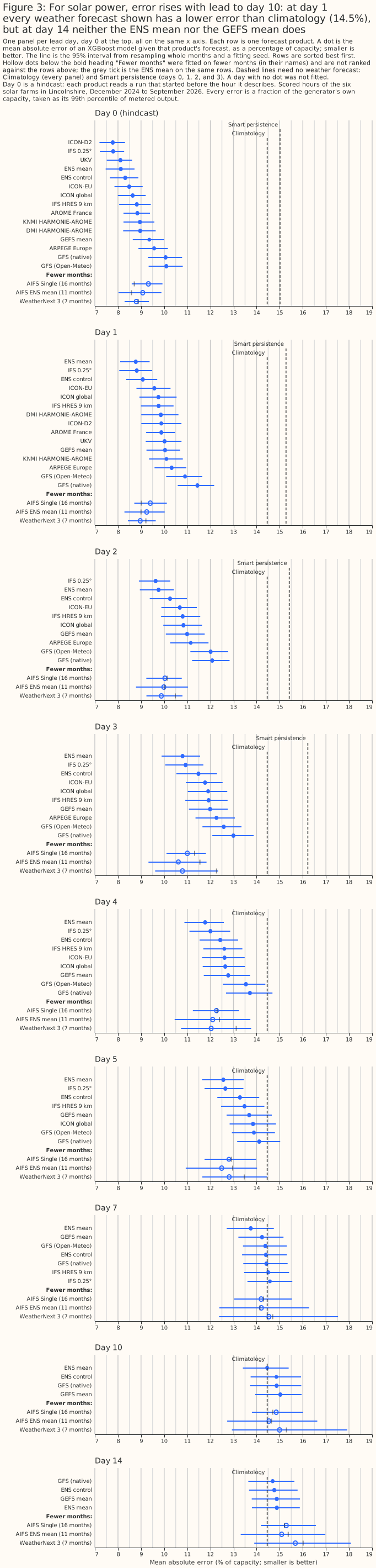
Figure 3: For solar power, error rises with lead to day 10: at day 1 every weather forecast shown has a lower error than climatology, a forecast that uses no weather data (14.5%), but at day 14 neither the ENS mean nor the GEFS mean does. Each panel is one lead day, from day 0 at the top, on one shared x axis, and each row is one forecast product, sorted best first. Among the full-window products, the ENS mean and IFS 0.25° have the lowest day-1 errors. Every full-window product except IFS HRES 9 km is scored on exactly the same hours, and IFS HRES 9 km is scored without the target days its archive lacks. The three rows below the heading "Fewer months" are fitted on fewer months: WeatherNext 3 (7 months, February to September 2026, no May rows), AIFS Single (16 months), and AIFS ENS mean (11 months). Their dots are hollow, they are not ranked against the rows above, and each has a grey tick for the ENS mean on the same rows. Figure 19 splits the WeatherNext 3 rows. At days 7 and 14 WeatherNext 3's solar error is not the lowest plotted: the ENS mean (13.7% at day 7) and GFS native (14.7% at day 14) are lower, on more months. Against the ENS mean on the same rows (14.7% and 16.0%) the difference is not resolved. Leads are not equal, which favours a product read from Open-Meteo's archive of past forecasts (Previous Runs), because it reads a fresher run than ENS on most hours (Limitations). Smart persistence, which uses no weather forecast, is drawn only at days 0 to 3, where it was scored. A lead day with no mark was not fitted, because it is beyond the product's forecast range or not in the archive we hold; nothing is filled in. Day 0 is a hindcast, not a day-ahead forecast a service could read.

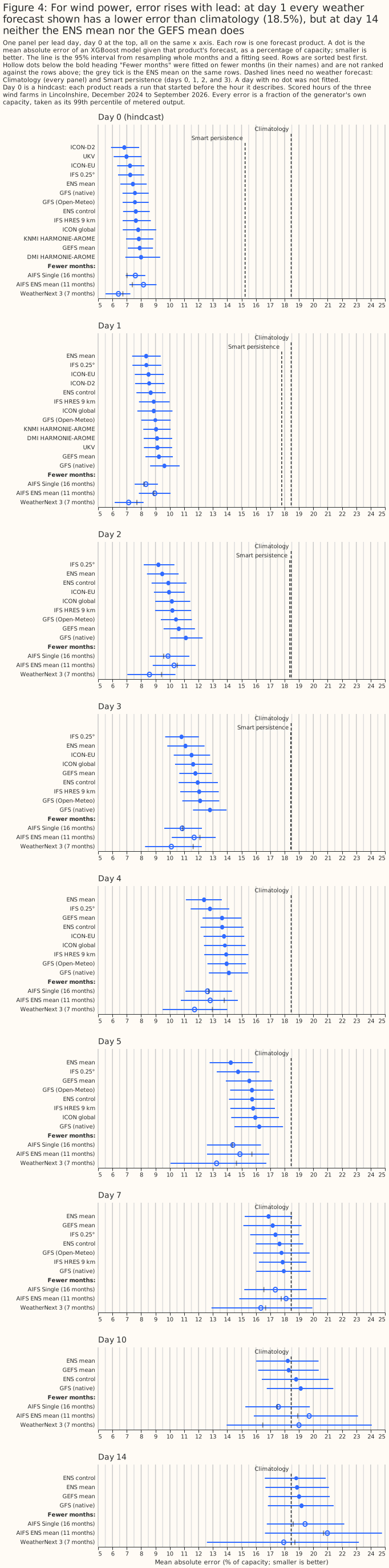
Figure 4: For wind power, error rises with lead: at day 1 every weather forecast shown has a lower error than climatology (18.5%), but at day 14 neither the ENS mean nor the GEFS mean does. The marks, rows, and limits are as in Figure 3, except as follows. At days 7 and 14, against the ENS mean on the same rows (16.7% and 18.7%), no difference from WeatherNext 3 is resolved, and the plotted ranks compare different row sets (Figure 20 splits the rows). At day 14 WeatherNext 3's 17.9% is not detectably below the shuffled-weather arms (18.3% and 18.6%), so the chart does not show that WeatherNext 3 beats the 18.5% climatology. The grey tick is the ENS mean of wind speed, not the ENS mean-vector reference matched to WeatherNext 3, which the WeatherNext 3 results section compares. Overlapping intervals can still hide a significant paired difference (Figure 6). The WeatherNext 3 row drops the hour ending 00:00 UTC at day 0, for which the WeatherNext 3 store holds no lead.

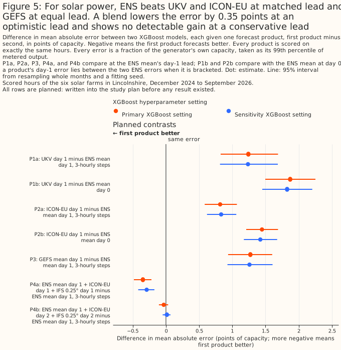
Figure 5: For solar power, ENS beats UKV and ICON-EU at matched lead and GEFS at equal lead. A blend lowers the error by 0.35 points at an optimistic lead and shows no detectable gain at a conservative lead.

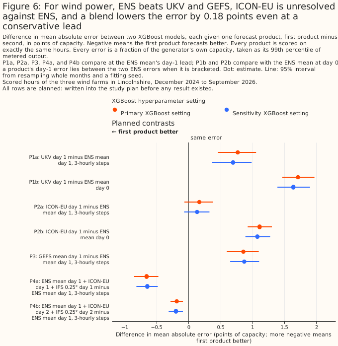
Figure 6: For wind power, ENS beats UKV and GEFS, ICON-EU is unresolved against ENS, and a blend lowers the error by 0.18 points even at a conservative lead.

How this page was made. The research question came from a human. Everything else — the code behind every result, the analysis, the figures, and the text — was written by Claude, Anthropic's AI model (for this page, Claude Opus 5, Claude Opus 5.5, and Claude Sonnet 5, with Claude Opus 5.5 and Claude Sonnet 5 also reusing shared code that Claude Opus 5 wrote). Several independent Claude reviewers have checked the method, the evidence, and the prose adversarially.

This study uses only Flexpectation's own data, and its purpose is to inform Flexpectation's choices. The study scores each weather product only at the 6 solar farms and 3 wind farms in Flexpectation's trial area in Lincolnshire. The study does not compare results across many regions or climates, so a result on this page may not hold elsewhere.

Key findings

Every finding is about each product as this study reads it, at 6 solar farms and 3 wind farms, and is not a ranking of the weather models behind the products. UKV, ICON-EU, and IFS 0.25° are single runs read at one grid point, and ENS and GEFS are ensemble means (Introduction).

In Figures 1 and 2, six products score a higher error than the ENS mean at lead days 1 to 5, for both solar and wind, every interval excluding zero. The six are IFS HRES 9 km, the GEFS mean, GFS (read natively and through Open-Meteo, a service that archives past weather forecasts), ICON global (the German weather service's global ICON), and the ENS control member, scored on 21 months. The excess runs from +0.306 points (the ENS control member, solar day 1) to +2.667 points (native GFS, solar day 1). By day 14, the GEFS mean, native GFS, and the ENS control member cannot be separated from the ENS mean for either technology.

Among the 114 product-by-day dots across both technologies on the 21-month rows at days 1 to 14, one has a lower error than the ENS mean with an interval clear of zero: IFS 0.25° for wind at day 2, at -0.268 points [-0.451, -0.089]. Chance alone could produce one clear dot of 114, and IFS 0.25°'s shorter lead favours it. At day 0, which a live service cannot use, ICON-D2 (the German weather service's regional ICON) and IFS 0.25° score a lower error for both technologies, and UKV and ICON-EU do for wind.

For WeatherNext 3 (WN3), Google's machine-learned weather model, AIFS Single, and AIFS ENS mean, the result depends on which ENS mean forms the zero line. The table gives each product's difference from ENS's mean, in points, against an XGBoost model given the ENS mean and fitted again on only the product's own months (the filled dot), and against the one fitted on all 21 months, scored on the same hours (the hollow mark).

Product (months)	Against the refitted ENS mean	Against the 21-month ENS mean
WeatherNext 3 (7, dashed intervals)	Lower at solar days 1 to 5 (day 1: -0.243 [-0.440, -0.069]) and wind days 0 to 5. Higher at wind day 10 (+1.652 [+0.014, +3.502]), where the weather scored no better than shuffled weather: the cause is not established, and the result is not evidence that WeatherNext 3 loses skill	Not distinguishably lower at those days. Higher at solar day 0 (+0.482 [+0.141, +0.886]), wind day 4 (+0.665 [+0.307, +1.004]), and wind day 10 (+2.714 [+0.885, +5.437])
AIFS Single (16)	Higher at day 0 and at solar day 1 (+0.391 [+0.171, +0.598]), and at wind day 7 (+0.800 [+0.015, +1.586]) and day 14 (+0.827 [+0.212, +1.460]). Every other interval at days 2 to 10 includes zero	Wind also higher at day 1 (+0.404 [+0.152, +0.665]), day 2 (+0.878 [+0.269, +1.700]), and day 5 (+0.642 [+0.110, +1.173])
AIFS ENS mean (11)	Higher at day 0 and at solar day 1 (+0.242 [+0.018, +0.478]). Lower at solar day 3 (-0.932 [-1.681, -0.312]), wind day 4 (-0.982 [-1.826, -0.303]), and wind day 5 (-0.831 [-1.535, -0.159])	Every mark at solar day 3, wind day 4, and wind day 5 includes zero

For WeatherNext 3's 7 months, the refitted ENS mean scores a higher error than the 21-month ENS mean (solar day 1: +0.539 points [+0.085, +1.194]), so a lower error than the refitted mean may reflect the weaker zero line. The weather-model version behind WeatherNext 3's archive is undocumented, so February to June may overlap WeatherNext 3's training data. Only the 3 months July to September postdate that training data, so the pooled 7 months are not a fair comparison.

Error rises with lead, and from day 10 the ENS mean is no better than climatology (Figures 3 and 4). At day 7 the ENS mean's error is lower than climatology's, though the solar gain lies near the 5% line with no second-setting check.

Mean absolute error, % of capacity	ENS mean, day 1	ENS mean, day 14	Climatology
Solar	8.771% [8.096, 9.373]	14.876% [13.797, 15.870]	14.458% [13.205, 15.592]
Wind	8.350% [7.373, 9.364]	18.867% [16.664, 21.091]	18.460% [16.341, 20.389]

Five limits apply to every dot in Figures 1 and 2. They are the same-rows zero line, the fresher run that most products read (so a lower error than ENS's is not evidence of skill at equal lead), day 0 being a hindcast, dashed intervals that are too narrow, and rows that are not independent tests, among which about 1 in 20 comparisons with no true difference is statistically significant at the 5% level by chance (Limitations).

Two limits apply to the Summary's blend and ENS-advantage results. Every solar blend control is itself worse than ENS alone, so the solar blend gain is not shown to come from the added weather (blending). Part of ENS's wind advantage may be timing noise that averaging removes (gaps).

Introduction

The question is which weather forecast, or blend of forecasts, gives the most accurate day-ahead power forecast at the 6 solar farms and 3 wind farms. Flexpectation's live service reads ENS at 09:00 UTC, so the answer decides whether a second weather source is worth ingesting. ENS is the incumbent. The table sets out each product a headline contrast uses, plus ICON-D2. The other products in the study are exploratory, and their results start at Error and lead.

Product	Lead at day 1, in hours after the run starts	Grid	Domain (the study reads Great Britain)	Archive read from	Delivery
ECMWF ENS, mean of 51 members	24 + h	About 9 km native, served on 0.25° cells; the study averages the cells overlapping each generator's H3 cell	Global	2024-04-01	Not measured; the study assumes the 00 UTC run is readable at 09:00 UTC
NOAA GEFS, mean of 31 members	24 + h	0.25°; the study reads the nearest cell	Global	2020-10-01	Not measured; the study assumes the 00 UTC run is readable at 09:00 UTC
UKV	24 + (h mod n)	1.5 km over the UK, served at 2 km	UK	2024-08-06	About 4 hours after the run starts
ICON-EU	24 + (h mod n)	6.5 km, served at about 7 km	Europe	2024-01-19	About 3.5 hours after the run starts
ICON-D2 (exploratory only)	24 + (h mod n)	2.2 km, served at about 2 km	Germany and neighbouring countries, not all of Great Britain	2024-01-19	About 1.5 hours after the run starts
IFS 0.25°	24 + (h mod n)	About 9 km native, served at 0.25°	Global	2024-03-06	Not measured

IFS 0.25° is the open-data 0.25° version of ECMWF's single high-resolution forecast run (HRES), not a member of ENS.

ICON-D2 covers Germany and neighbouring countries, ICON's 100 m wind is a derived value, and ENS at a generator is a smoothed mean. ICON-D2 is the German weather service's 2.2 km ICON configuration for Germany and neighbouring countries. ICON-EU's, ICON-D2's, and ICON global's served "100 m" wind speed is Open-Meteo's derivation, the 120 m speed multiplied by about 0.98, and not a product of the German weather service. ENS at a generator is the mean of the 0.25° grid cells that overlap the generator's H3 resolution-5 hexagon (about 253 km²), weighted by overlap. That mean is a smoothed value, whereas each Previous Runs product is read at a single grid point.

In the table, h is the UTC hour of the row and n is the interval between runs of a product's weather model. ENS and GEFS start one run per day, at 00 UTC. UKV, ICON-EU, and IFS 0.25° reach the study through Open-Meteo's Previous Runs archive, whose lead depends on n (How the leads are matched). The scored rows start on 2024-12-01, after the archive start date of every product in the table. The grids, coverage, and delivery times of UKV, ICON-D2, and ICON-EU come from the past-wind study, which measured the delivery times for a different purpose. The archive start dates come from the weather-products survey. The study did not measure the delivery time of ENS, GEFS, or IFS 0.25°, and ECMWF's published dissemination schedule was not checked against the 09:00 UTC assumption.

Data and methods

How the leads are matched

Open-Meteo's Previous Runs archive is not a fixed-lead instrument, so the study cannot compare its products with ENS at one lead. A value labelled previous_dayN comes from the freshest run of the weather model that was initialised at least N × 24 hours before the hour it describes. For a weather model that starts a run every n hours, the lead of that value is 24N + (h mod n) hours, where h is the UTC hour of day. The lead therefore differs between products. No Previous Runs value reproduces a forecast issued at a fixed time each day.

A check against GFS runs on two days supports the run-selection rule, and the same check found no clear run cycle for UKV. The study's verification script (V1) checked this run-selection rule against GFS runs on two days (2025-07-01 and 2025-07-02) at the nine generators, and the check passed. Served 100 m wind speed differed from the run initialised exactly 24N hours before the hour by a mean absolute difference of 0.102 km/h at N = 1 and 0.100 km/h at N = 2, against 0.416 and 0.515 km/h for a run one hour older. Served radiation matched a run chosen by the hour's label (a mean absolute difference of 4.96 W/m² at N = 1) better than a run chosen by the hour's start (21.94 W/m²).

The rule for every other product rests on the assumption that Open-Meteo applies one rule to every weather model. For UKV, the run-switch check (V1b) found no clear run cycle: the check's score was 1.07 for wind and 1.10 for temperature, and a cycle needs a score of 1.3. The study therefore reports, for solar, the share of hours whose rebuilt radiation value, which the next paragraph explains is built from two hourly snapshots, would straddle a run change under two assumed cycles: 33.3% at a 3-hour cycle and 16.9% at a 6-hour cycle.

UKV's hourly solar radiation is the study's own rebuild from two snapshots, so the solar gap between UKV and ENS includes the effect of that rebuild. The radiation timestamp check gave a median peak offset of -13 minutes for UKV, the offset a snapshot taken at the hour's label gives. Every other product measured -28 to -35 minutes, the offset an hour-ending mean gives. The study rebuilds UKV's hourly radiation from its hourly snapshots at offsets (-60, 0) minutes. The rebuild gives a median peak of -43 minutes, the offset of an hour-ending mean, and the timestamp check agrees with the rebuild. The study chose the two offsets by the timestamp check alone, and did not compare UKV's error under any other rebuild.

If Open-Meteo fills a missing run with an older run, a row's lead can exceed the lead the rule gives, and a longer lead would weaken the upper side of the bracket. The upper side needs each product's lead to be no longer than ENS day N's. On a filled row the product's lead is longer, so its error could exceed ENS day N's because of the run's age and not because of the weather model. The V1 check compared GFS with runs on two days only, so the study cannot rule out a fill for any product.

ENS and GEFS are compared at exactly matched lead, because both are whole-run archives. Each ensemble contributes its 00 UTC run, read as though at 09:00 UTC on the run's day. A forecast for day d is the run's forecast for the calendar day d days after the run, so a row's lead is 24d + h hours for both ensembles. The study assumes both runs were readable by 09:00 UTC, which is when the live service reads its ENS run, and did not measure when either run was published. The GEFS contrast, P3, is therefore the only planned contrast whose two arms have exactly the same lead on every row.

ENS at day N−1 and at day N brackets each Previous Runs product at day N. On a row for hour h, ENS day N−1 has lead 24(N−1) + h hours, which is shorter than the product's 24N + (h mod n). ENS day N has lead 24N + h, which is at least as long. If a product's error is lower than ENS day N−1's error, the product beats ENS even though ENS had the shorter lead. If a product's error is higher than ENS day N's error, ENS beats the product even though the product's lead was no longer. The study calls the first contrast the lower side of the bracket (P1b for UKV, P2b for ICON-EU) and the second contrast the upper side (P1a and P2a). The bracket needs no knowledge of a product's run cycle n.

ENS day 0 is a bracket side only. A service issuing at 09:00 UTC cannot deliver a forecast whose early hours have already passed, so ENS day 0 is never offered as a product.

A product beats ENS, loses to ENS, or is unresolved, and a verdict stands only if both XGBoost settings give it. These three verdicts were fixed in the plan before any fit:

• Beats ENS at matched lead: the lower-side difference is negative and significant at the 5% level.
• Loses to ENS at matched lead: the upper-side difference is positive and significant at the 5% level.
• Unresolved at matched lead: neither of those two conditions holds, so the product's error lies between the two ENS errors, and the study cannot place the product's error more precisely.

"Beats" needs a product to beat ENS at day N−1, not at day 0, and "loses" is easier to reach than "beats" by construction. For a product at day N, ENS at day N−1 has a lead 24 − (h − (h mod n)) hours shorter than the product's, and ENS at day N has a lead h − (h mod n) hours longer. Averaged over the 24 UTC hours, for a product whose runs start every 6 hours, ENS at day N−1 has a lead 15 hours shorter and ENS at day N has a lead 9 hours longer. The "loses" test therefore sits closer to a matched lead than the "beats" test does, and gives ENS a smaller handicap. Both tests are conservative, but the "beats" test is the more conservative one. A product a little worse than ENS is therefore likelier to reach "loses" than a product a little better than ENS is to reach "beats".

A verdict that the two settings disagree on is unresolved, and only the planned contrasts carry headline claims, which are the claims in the Summary. The page shows both settings. The planned contrasts are P1a, P1b, P2a, P2b, P3, P4a, and P4b (the blends of ENS with ICON-EU and IFS 0.25° at day 1 and at day 2), and the two blend guards per technology (each blend minus its permutation control). All of the planned contrasts were written into the study plan before any result existed. The split between planned and exploratory contrasts applies to the contrast tables and to the headline claims: every contrast outside the planned list is exploratory, and so is any number that a paragraph quotes from an exploratory table. Analyses added after a result was seen, such as the two single-product wind blends, are exploratory and also post hoc. An exploratory interval with no real effect behind it has a nominal 5% chance of being statistically significant at the 5% level, and a higher chance if the intervals are too narrow (Limitations says how far the intervals can be trusted).

The bracket assumes that ENS's own error does not fall as its lead lengthens, and the study tests that assumption band by band. For each day pair the study uses (day 0 to 1, 1 to 2, and 2 to 3) and for each 3-hour band of UTC hours, the study computes the change in ENS's error. A band whose point estimate is zero or below is voided. Every bracket that rests on that day pair loses the voided band. The rule reacts to noise, because a point estimate can fall to zero or below by chance where the interval contains zero. The check tests only ENS's own error, so it does not test whether the Previous Runs archive follows the lead rule above, and it does not test any product's error at all.

The solar and wind sections give the result of this check.

The XGBoost model, the scored hours, and the folds

Every arm is the same XGBoost model given the same kinds of column, and only the weather product differs. The XGBoost model is fitted separately for each generator with an absolute-error objective and three fitting seeds (0, 1, and 2). Forecasts are scored out of fold. Curtailed hours are left out of training and kept for scoring. Every prediction is held to the generator's export cap. Column subsampling is switched off (colsample_bytree is 1), because a wider arm otherwise wins without carrying more information. Each single-product arm has seven columns:

• Solar: hour of day, day of year, an era code, the sun's elevation and azimuth, and the product's global horizontal irradiance and 2 m air temperature at its own lead.
• Wind: hour of day, day of year, an era code, and the product's wind speed at 100 m, the sine and cosine of its 100 m wind direction, and its 10 m wind speed at its own lead.

A blend has more columns than a single-product arm, so each blend has a control with the same column count. The solar blend has 11 columns and the wind blend has 15. ENS's columns stay real in the control. Each other product's weather columns are replaced by values shuffled among the hours that share a generator, a year-month (a calendar month of one year, such as 2025-03), and a UTC hour of day, so no shuffled value crosses a fold. A wind product's direction sine and cosine move together under one shuffle, and every other column is shuffled separately. The blend minus its control separates the effect of the other products' weather from the effect of the extra columns.

Scoring is on the same hours for every arm, except IFS HRES 9 km and the AIFS arms. Every other arm is scored on the rows where the target, the no-weather baselines, and every planned product are present. IFS HRES 9 km loses the target days its archive lacks, and the AIFS arms have rows of their own (the extra arms and How AIFS is read). A row is one hour at one generator. Solar has 39,030 candidate rows from 2024-12-01 and 35,263 shared rows. Wind has 42,144 candidate rows and 37,407 shared rows.

Requiring a UKV day-1 value removes the most rows, so the shared rows hold little of spring 2026 (Limitations gives the counts).

Exploratory arms other than IFS HRES 9 km and the AIFS arms are fitted on the same rows with their few missing values left as missing, which XGBoost handles natively (Limitations gives the shares).

The shared rows cover 21 year-months.

Folds are whole months, cut inside three eras, and the study prints which months no fold can cover. The eras end at 2025-10-01 and at the Met Office's UKV upgrade on 2026-01-21. The part month around the upgrade is dropped. Five folds of whole months are cut inside each era. The third era's folds are rotated by three fold positions (NWP_ERA_FOLD_OFFSETS = {0: 0, 1: 0, 2: 3}) so that no calendar month is held out of every era at once. A rotation of 3 is the first rotation search_fold_offsets returns that covers every month in both technologies. search_fold_offsets reads only which hours exist and ran before any XGBoost model was fitted, so no forecast error informed the rotation. The 2025-10-01 cut comes from the shared fold helper and is harmless here. IFS Cycle 50r1 (2026-05-12) is not an era cut.

Every arm gets the same era code. Of 124 solar (site, fold, month) cells, 20 are not covered by training, and of 63 wind cells, 9 are not covered. Every uncovered cell is a calendar month that occurs in one year only at that site, so no other fold holds that month and training never sees the season.

Every error is divided by its own generator's capacity before any mean or difference, and every interval resamples whole year-months. Capacity is the generator's effective_capacity_mw, its 99th percentile of metered output, as defined on the blending page. Each of 2,000 resamples draws whole year-months, and one of the three fitting seeds, paired across the two arms of a contrast. Each contrast asserts that both arms hold the same rows. The XGBoost model is fitted at two hyperparameter settings, called primary and sensitivity. The page shows the sensitivity setting for every planned contrast, for the exploratory results that decide whether a planned contrast is informative (the permutation controls against ENS alone, and the check that ENS's error rises with lead), and for any exploratory result near the 5% line, meaning a result with a 95% interval bound within 20% of the interval's width from zero. Every other exploratory result is shown at the primary setting only. The extra lead-day and day-0 arms below have no sensitivity fit, so about 40 of their results that lie near the 5% line have no second-setting check. Among them are the ENS mean's gain over climatology at day 7 for solar (-0.710 [-1.398, -0.064]), IFS 0.25° minus ENS at day 5 for wind, and ICON-D2 minus ICON-EU at day 1 for solar.

The extra lead days, day 0, and the products added later

Every extra arm is exploratory, is fitted at the primary setting only, and is read on the same shared rows, folds, and eras as the planned arms, with two exceptions. IFS HRES 9 km loses the target days its archive lacks, and the AIFS and WeatherNext 3 arms have rows of their own. The companion page says how each extra product is read: the lead days and day 0, AIFS, WeatherNext 3, and why the WeatherNext 3 months before July may overlap its training data.

Results

The XGBoost models track measured output, and every day-1 weather forecast beats climatology

The XGBoost models track the measured output at every farm, so contrasts of a few tenths of a point are contrasts between working forecasts. Figure 7 shows out-of-fold day-1 forecasts given ENS against the measured output at all six solar farms, and Figure 8 shows the same for the three wind farms. Each figure covers one week, chosen by a stated rule from the measured output alone. For solar, the rule takes the week whose daily mean output varies most from day to day. For wind, the rule takes the week with the largest mean hour-to-hour change in output. Only weeks in which every generator has scored hours on all seven days qualify.

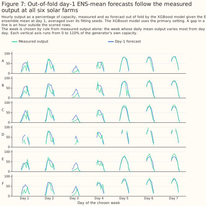
Figure 7: Out-of-fold day-1 ENS-mean forecasts follow the measured output at all six solar farms.

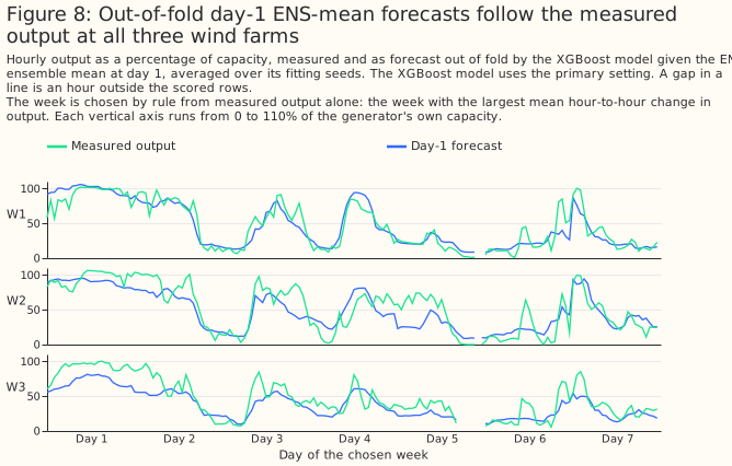
Figure 8: Out-of-fold day-1 ENS-mean forecasts follow the measured output at all three wind farms.

At day 1, an XGBoost model given ENS beats climatology by a wide margin. Given ENS's day-1 mean, the error is 8.766% of capacity [8.096, 9.355] for solar and 8.427% [7.444, 9.503] for wind. The climatology baseline scores 14.458% [13.205, 15.592] for solar and 18.460% [16.341, 20.389] for wind. Climatology is the median output at each generator for each calendar month and hour of day over the training folds.

Persistence baselines do no better than climatology on solar, and smart persistence (the last day's clear-sky index applied to clear-sky irradiance for solar, persistence blended with climatology for wind) beats climatology on wind (exploratory). Smart persistence at day 1 scores 15.274% [14.251, 16.272] on solar and 17.799% [15.824, 19.614] on wind. Smart persistence's error minus climatology's is +0.816 points [+0.040, +1.609] on solar and -0.662 points [-0.946, -0.390] on wind.

A baseline for a day-1 to day-3 forecast reads only telemetry up to 09:00 UTC on the run's day, the same information the live service has. A baseline for the run's own day (day 0) reads telemetry only up to the run's 00 UTC initialisation time. Figures 3 and 4 draw climatology and day-1 smart persistence only. Solar persistence on the run's own day (persistence_day0) would repeat the last observed hour, a night-time value near zero, across the whole day.

Overlapping intervals in Figures 3 and 4 do not mean two products are equal. The errors of all the products rise and fall together from month to month, and pairing the two arms of a contrast cancels that shared swing. The paired differences in Figures 5 and 6 are the test of which gaps are statistically significant.

Figures 3 and 4 favour the Previous Runs products, because their day-1 leads are shorter than ENS's on most hours, so their ordering against ENS is not an ordering at equal lead. Only GEFS has ENS's exact lead on every row, and IFS 0.25° day 1 can also come from a newer ECMWF run than ENS's 00 UTC run (How the leads are matched).

Error rises with lead, and from day 10 the ENS mean is no better than climatology (exploratory)

Every product's error rises with lead, up to day 10 where a product is fitted that far, the ENS mean's error is lower than climatology's at day 7, and from day 10 the ENS mean's error cannot be told apart from climatology's. Every mark in this section is a GPU fit. The ENS mean's errors at days 1 and 14, and climatology's, are in the Key findings table. The table below gives the other days.

ENS mean error, % of capacity	Day 5	Day 7	Day 10
Solar	12.560% [11.639, 13.448]	13.748% [12.706, 14.745]	14.457% [13.406, 15.388]
Wind	14.251% [12.774, 15.777]	16.884% [15.218, 18.527]	18.223% [16.022, 20.367]

Paired with climatology, the ENS mean is -0.710 [-1.398, -0.064] points for solar and -1.577 [-2.713, -0.460] points for wind at day 7, so the study shows a gain over climatology at day 7. At day 10 the differences are -0.001 [-0.556, +0.531] and -0.238 [-1.315, +0.812], and at day 14 they are +0.418 [-0.325, +1.108] and +0.406 [-0.571, +1.341], so the study shows neither a gain nor a loss at those leads. The day-14 wind marks may sit 0.04 to 0.09 points below where a CPU fit would put them, a difference that would change neither conclusion.

No product fitted at day 10 or day 14 has an error that can be told apart from climatology's. The table gives every arm fitted at those leads, and the ENS mean and GEFS at day 7 for comparison.

Exploratory: arm minus climatology (points, primary)	Solar	Wind
ENS mean, day 7	-0.710 [-1.398, -0.064]	-1.577 [-2.713, -0.460]
GEFS mean, day 7	-0.224 [-0.906, +0.396]	-1.286 [-2.508, -0.183]
ENS mean, day 10	-0.001 [-0.556, +0.531]	-0.238 [-1.315, +0.812]
GEFS mean, day 10	+0.569 [-0.148, +1.193]	-0.172 [-1.137, +0.738]
ENS control member, day 10	+0.398 [-0.346, +1.022]	+0.342 [-0.790, +1.445]
GFS (native), day 10	+0.409 [-0.291, +1.031]	+0.669 [-0.203, +1.641]
ENS mean, day 14	+0.418 [-0.325, +1.108]	+0.406 [-0.571, +1.341]
GEFS mean, day 14	+0.416 [-0.231, +1.026]	+0.550 [-0.353, +1.414]
ENS control member, day 14	+0.307 [-0.471, +0.992]	+0.349 [-0.511, +1.140]
GFS (native), day 14	+0.238 [-0.431, +0.825]	+0.724 [-0.225, +1.623]

The error of the ENS mean, the ENS control member, GEFS, and native GFS rises in every step from day 5 to day 10, with one exception, and by day 14 the rise has stopped for most of them. For solar, native GFS's day 7 minus day 5 is +0.311 [-0.075, +0.701] points, the one step whose interval includes zero. From day 10 to day 14 the ENS mean's solar error and GEFS's wind error still rise, and every other arm's error does not rise detectably.

Exploratory: day 14 minus day 10, same product (points, primary)	Solar	Wind
ENS mean	+0.419 [+0.090, +0.714]	+0.644 [-0.008, +1.292]
GEFS mean	-0.153 [-0.422, +0.105]	+0.722 [+0.193, +1.273]
ENS control member	-0.091 [-0.309, +0.115]	+0.007 [-0.763, +0.727]
GFS (native)	-0.171 [-0.431, +0.069]	+0.055 [-0.291, +0.384]

The ENS control member has a higher error than the ENS mean at every fitted day from 0 to 10, and the two cannot be told apart at day 14. The ENS control member is one run of the ensemble at the ENS mean's own lead, so the difference measures what averaging the members adds. The day-1 difference is in Part of ENS's advantage is ensemble averaging and timing.

Exploratory: ENS control member minus ENS mean (points, primary)	Solar	Wind
Day 0	+0.190 [+0.111, +0.267]	+0.201 [+0.126, +0.282]
Day 2	+0.496 [+0.303, +0.698]	+0.424 [+0.255, +0.601]
Day 3	+0.687 [+0.401, +0.991]	+0.854 [+0.606, +1.130]
Day 5	+0.721 [+0.297, +1.217]	+1.487 [+1.028, +1.891]
Day 7	+0.656 [+0.292, +0.998]	+0.764 [+0.155, +1.485]
Day 10	+0.399 [+0.079, +0.716]	+0.580 [+0.210, +0.968]
Day 14	-0.110 [-0.329, +0.108]	-0.057 [-0.575, +0.377]

GEFS has a higher error than the ENS mean at days 5, 7, and 10 for solar and at day 5 for wind, and cannot be told apart from the ENS mean at any other of the days 5 to 14 fitted. GEFS and ENS have the same lead on every row. GEFS minus ENS is +1.118 [+0.704, +1.569] points for solar and +1.290 [+0.804, +1.791] points for wind at day 5, +0.487 [+0.174, +0.820] and +0.290 [-0.496, +1.119] at day 7, +0.569 [+0.318, +0.810] and +0.065 [-0.432, +0.518] at day 10, and -0.002 [-0.284, +0.256] and +0.143 [-0.323, +0.560] at day 14.

At day 5, IFS 0.25° cannot be told apart from ENS for solar and is worse than ENS for wind, although its lead is shorter than ENS's on most hours. IFS 0.25° minus ENS at day 5 is +0.088 [-0.377, +0.575] points for solar and +0.507 [+0.081, +0.937] points for wind.

Solar, mean absolute error in % of capacity (primary setting). Every cell is a GPU fit, and each 95% interval is in the batch reports and in Figure 3. IFS HRES 9 km cells are scored on the shared hours minus the target days its archive lacks, and the other rows use every shared hour. "Not in archive" marks a lead day that the archive we hold does not carry, and "beyond horizon" marks a lead day past the product's forecast range:

Product	Day 0	Day 1	Day 2	Day 3	Day 5	Day 7	Day 10	Day 14
ENS mean	8.125	8.771	9.759	10.797	12.560	13.748	14.457	14.876
IFS 0.25°	7.793	8.815	9.633	10.930	12.648	14.577	not in archive	not in archive
ENS control member	8.315	9.076	10.255	11.484	13.281	14.404	14.856	14.765
ICON-EU	8.487	9.575	10.677	11.770	not in archive	not in archive	not in archive	not in archive
ICON global	8.637	9.752	10.834	11.904	13.846	not in archive	not in archive	not in archive
IFS HRES 9 km (Open-Meteo)	8.816	9.762	10.801	11.925	13.475	14.505	beyond horizon	beyond horizon
DMI HARMONIE-AROME	8.962	9.856	beyond horizon	beyond horizon	beyond horizon	beyond horizon	beyond horizon	beyond horizon
ICON-D2	7.776	9.877	beyond horizon	beyond horizon	beyond horizon	beyond horizon	beyond horizon	beyond horizon
AROME France	8.841	9.879	beyond horizon	beyond horizon	beyond horizon	beyond horizon	beyond horizon	beyond horizon
UKV	8.108	10.019	not in archive	not in archive	not in archive	not in archive	not in archive	not in archive
GEFS mean	9.357	10.039	10.993	11.987	13.679	14.234	15.027	14.874
KNMI HARMONIE-AROME	8.952	10.099	beyond horizon	beyond horizon	beyond horizon	beyond horizon	beyond horizon	beyond horizon
ARPEGE Europe	9.566	10.325	11.151	12.262	beyond horizon	beyond horizon	beyond horizon	beyond horizon
GFS (Open-Meteo)	10.094	10.902	12.011	12.579	13.884	14.378	not in archive	not in archive
GFS (native)	10.061	11.438	12.081	12.996	14.112	14.423	14.867	14.696

Wind, mean absolute error in % of capacity (primary setting). Every cell is a GPU fit, and each 95% interval is in the batch reports and in Figure 4. ARPEGE Europe and AROME France have no wind arm:

Product	Day 0	Day 1	Day 2	Day 3	Day 5	Day 7	Day 10	Day 14
ENS mean	7.426	8.350	9.473	11.089	14.251	16.884	18.223	18.867
IFS 0.25°	7.241	8.363	9.205	10.815	14.758	17.362	not in archive	not in archive
ICON-EU	7.224	8.516	9.946	11.515	not in archive	not in archive	not in archive	not in archive
ICON-D2	6.826	8.562	beyond horizon	beyond horizon	beyond horizon	beyond horizon	beyond horizon	beyond horizon
ENS control member	7.627	8.669	9.897	11.943	15.738	17.647	18.803	18.809
IFS HRES 9 km (Open-Meteo)	7.636	8.879	10.179	12.047	15.810	17.864	beyond horizon	beyond horizon
ICON global	7.799	8.882	10.142	11.626	15.956	not in archive	not in archive	not in archive
GFS (Open-Meteo)	7.568	8.988	10.430	12.110	15.724	17.786	not in archive	not in archive
KNMI HARMONIE-AROME	7.841	9.043	beyond horizon	beyond horizon	beyond horizon	beyond horizon	beyond horizon	beyond horizon
DMI HARMONIE-AROME	7.995	9.110	beyond horizon	beyond horizon	beyond horizon	beyond horizon	beyond horizon	beyond horizon
UKV	6.979	9.136	not in archive	not in archive	not in archive	not in archive	not in archive	not in archive
GEFS mean	7.899	9.241	10.626	11.781	15.541	17.174	18.288	19.010
GFS (native)	7.567	9.622	11.117	12.798	16.233	17.946	19.129	19.184

Day 0 is lower than day 1 for every product, and ICON-D2's day 0 is the lowest (exploratory)

At day 0, ICON-D2 has the lowest wind error of any forecast fitted and ties with IFS 0.25° for the lowest solar error (Figures 3 and 4), and every product's day-0 error is lower than its own day-1 error. Day 0 is a hindcast that a service issuing at 09:00 UTC could not read, and the comparison with ENS at day 0 favours the Previous Runs products, which read the freshest run. The companion page holds the day-0 errors, the day-0 differences from ENS, and the check of the served lead.

For solar power, ENS beats UKV and ICON-EU at matched lead and GEFS at equal lead

For solar power, no product tested beats the European Centre for Medium-Range Weather Forecasts ensemble (ENS) at matched lead: UKV and ICON-EU both lose, at both XGBoost hyperparameter settings. Every difference below is the mean absolute error of an XGBoost model given the first product, minus the error of an XGBoost model given the second, in percentage points ("points") of capacity, with a 95% interval. A positive difference means the first product forecasts worse. UKV is the Met Office's UK weather model. ICON-EU is the European domain of the German weather service's ICON weather model.

A Previous Runs product cannot be given ENS's exact lead, so each product is bracketed between ENS at day 0 and ENS at day 1. How the leads are matched defines the bracket, the three verdicts, and which contrasts are planned. Every other contrast on this page is exploratory.

Contrast (solar, points)	Primary setting	Sensitivity setting
P1a: UKV day 1 − ENS day 1 (upper side)	+1.242 [+0.824, +1.689]	+1.236 [+0.815, +1.686]
P1b: UKV day 1 − ENS day 0 (lower side)	+1.872 [+1.497, +2.252]	+1.826 [+1.451, +2.205]
P2a: ICON-EU day 1 − ENS day 1 (upper side)	+0.817 [+0.584, +1.069]	+0.832 [+0.619, +1.060]
P2b: ICON-EU day 1 − ENS day 0 (lower side)	+1.447 [+1.210, +1.689]	+1.422 [+1.174, +1.676]
P3: GEFS day 1 − ENS day 1 (equal lead)	+1.272 [+0.937, +1.601]	+1.259 [+0.927, +1.606]

Both sides of both brackets are positive and significant, so UKV and ICON-EU have a higher error than ENS even at ENS's shorter day-0 lead. The verdict for each product is "loses" at the primary setting and at the sensitivity setting. At the primary setting the XGBoost model given ENS at day 1 has an error of 8.766% of capacity [8.096, 9.355], against 10.009% [9.178, 10.750] for UKV and 9.583% [8.819, 10.290] for ICON-EU. ENS at day 0 has an error of 8.137% [7.475, 8.728]. ENS at day 0 is a bracket side only, because a service issuing at 09:00 UTC cannot read a forecast for hours that have already passed.

The bracket rests on ENS's error rising with lead, and that assumption fails in one band of hours for solar power. From day 0 to day 1 the ENS error changes by -0.025 points [-0.133, +0.051] in the band 03-06 UTC at the primary setting, and by -0.019 points [-0.155, +0.106] at the sensitivity setting, so the study voids every bracket in that band. The sensitivity setting checks the day-0-to-day-1 pair only. Within that band each product's own bracket is unresolved: for UKV the lower side is -0.013 [-0.088, +0.092] and the upper side is +0.012 [-0.100, +0.145] at the primary setting (exploratory). Dropping the voided band from the rows leaves the upper sides positive: +1.261 [+0.840, +1.715] for UKV and +0.828 [+0.595, +1.075] for ICON-EU at the primary setting, from 34,735 rows. UKV's lower side is +1.901 points [+1.527, +2.284]. UKV and ICON-EU therefore still lose (exploratory). In every other band of the day-0-to-day-1 pair, the point estimate is positive at both settings. Within the day-0-to-day-1 pair, the interval is above zero in all but the band 18-21 UTC, where the change is +0.036 points [-0.062, +0.125] at the primary setting and +0.062 points [-0.048, +0.175] at the sensitivity setting. The point estimate for the band 18-21 UTC is positive, so the study does not void the band. In every band of the pairs day 1 to 2 and day 2 to 3, the point estimate is positive at the primary setting.

At equal lead the solar test of ICON-EU has too few rows to separate the products. ICON-EU's day-1 lead equals ENS day 1's on hours 00-05 UTC, but the shared solar rows in that window fall at 05 UTC only. On those 528 rows in 8 months, ICON-EU minus ENS at day 1 is +0.092 points [-0.056, +0.269] (exploratory). The verdict for ICON-EU therefore rests on the bracket.

ENS also beats GEFS, the free ensemble from the US National Oceanic and Atmospheric Administration (NOAA), at exactly equal lead. GEFS is the Global Ensemble Forecast System. GEFS and ENS have the same lead on every row, so the P3 contrast needs no bracket. The XGBoost model given the GEFS ensemble mean at day 1 has an error of 10.039% [9.234, 10.689] against 8.766% for ENS (P3 in the table).

The solar result holds at each of the six generators. The generators are labelled A to F. UKV minus ENS at day 1 (P1a) is positive and significant at every generator, from +1.087 points [+0.533, +1.649] at generator A to +1.442 points [+1.008, +1.918] at generator E. ICON-EU minus ENS at day 1 (P2a) is positive and significant at every generator too, from +0.668 points [+0.408, +0.966] at generator E to +1.075 points [+0.786, +1.375] at generator F. These contrasts are exploratory. Each interval resamples months and fitting seeds within one generator, so the interval does not cover differences between generators.

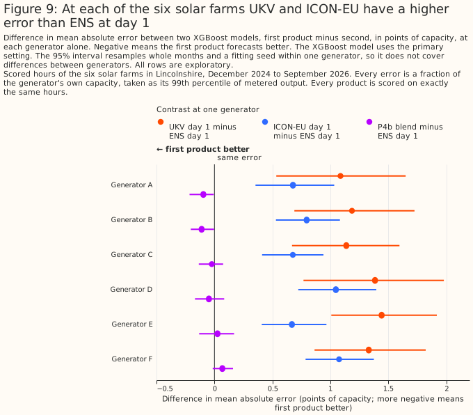
Figure 9: At each of the six solar farms UKV and ICON-EU have a higher error than ENS at day 1.

For wind power, ENS beats UKV and GEFS, and ICON-EU is unresolved against ENS

For wind power, UKV loses to ENS at matched lead, and ICON-EU is unresolved against ENS. The verdict for UKV is "loses" at both settings, and the verdict for ICON-EU is "unresolved" at both settings. The differences are defined in the solar section above, and the bracket in How the leads are matched. A positive difference means the first product forecasts worse.

Contrast (wind, points)	Primary setting	Sensitivity setting
P1a: UKV day 1 − ENS day 1 (upper side)	+0.770 [+0.460, +1.057]	+0.697 [+0.371, +0.987]
P1b: UKV day 1 − ENS day 0 (lower side)	+1.713 [+1.467, +1.970]	+1.640 [+1.391, +1.902]
P2a: ICON-EU day 1 − ENS day 1 (upper side)	+0.169 [-0.064, +0.384]	+0.134 [-0.069, +0.328]
P2b: ICON-EU day 1 − ENS day 0 (lower side)	+1.112 [+0.926, +1.305]	+1.077 [+0.890, +1.277]
P3: GEFS day 1 − ENS day 1 (equal lead)	+0.858 [+0.598, +1.099]	+0.872 [+0.652, +1.105]

ICON-EU is unresolved because its upper side includes zero while its lower side is well above zero. ICON-EU is not better than ENS at day 0 (P2b is positive and significant), and its difference from ENS at day 1 (P2a) has an interval that includes zero at both settings. The wind error of the XGBoost model given ENS at day 1 is 8.427% of capacity [7.444, 9.503] at the primary setting, against 9.197% [8.213, 10.279] for UKV and 8.595% [7.588, 9.707] for ICON-EU. ENS at day 0 has an error of 7.483% [6.566, 8.511].

For wind, ENS's error rises with lead in every band of hours, so no bracket is voided. The change from day 0 to day 1 is positive in all eight 3-hour bands at both settings, from +0.629 points [+0.331, +0.948] in the band 03-06 UTC to +1.203 points [+0.874, +1.546] in the band 15-18 UTC at the primary setting. The pairs day 1 to 2 and day 2 to 3 also have a positive point estimate in every band at the primary setting.

On hours 00-05 UTC, where the two leads are exactly equal, ICON-EU has a higher wind error than ENS (exploratory); hours 00-05 UTC are night hours, so the result need not hold for the rest of the day. ICON-EU's day-1 lead equals ENS day 1's on hours 00-05 UTC. On those 9,228 rows, ICON-EU minus ENS at day 1 is +0.540 points [+0.237, +0.840], against +0.169 points [-0.064, +0.384] over all hours. The contrast is +0.669 points [+0.378, +0.987] on the band 00-03 UTC (4,632 rows) and +0.410 points [+0.035, +0.761] on the band 03-06 UTC (4,596 rows). UKV's day-1 lead equals ENS day 1's on hour 00 UTC, where UKV minus ENS at day 1 is +1.278 points [+0.901, +1.697] on 1,540 rows. All of these contrasts are exploratory. The ICON-EU contrast on hours 00-05 UTC is positive and significant, unlike the unresolved bracket over all hours.

ENS also beats GEFS at exactly equal lead for wind (P3 in the table). The GEFS error is 9.285% [8.333, 10.273] at the primary setting.

UKV has a higher error than ENS at all three wind generators in the point estimates, but the difference is statistically significant at the 5% level at only two of the three generators, and at generator W3 the difference is +0.269 points [-0.463, +0.857]. The generators are labelled W1 to W3. UKV minus ENS at day 1 (P1a) is +1.128 points [+0.819, +1.475] at generator W1 and +0.893 points [+0.640, +1.161] at generator W2. At generator W3 the difference is +0.269 points [-0.463, +0.857]. ICON-EU minus ENS at day 1 (P2a) is +0.206 points [-0.041, +0.464] at W1, +0.303 points [+0.014, +0.585] at W2, and -0.012 points [-0.358, +0.319] at W3. These contrasts are exploratory. Each interval resamples months and fitting seeds within one generator, so the interval does not cover differences between generators.

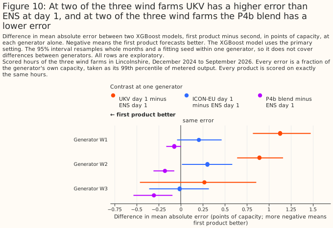
Figure 10: At two of the three wind farms UKV has a higher error than ENS at day 1, and at two of the three wind farms the P4b blend has a lower error.

A blend lowers the wind error at both leads tested, and the solar error only at an optimistic lead

A blend of ENS, ICON-EU, and IFS 0.25° lowers the wind error at both leads tested, and lowers the solar error only at the optimistic lead. Which single weather forecast should be added to ECMWF's ensemble mean first? compares blends of ENS with one product at a time.

Blend P4a adds ICON-EU and IFS 0.25° at their day 1 and blend P4b at their day 2, and P4b decides the verdict because a live service could have read every value it adds. Each blend gives one XGBoost model the ENS day-1 columns plus the ICON-EU and IFS 0.25° columns. Both blends are planned. Every value P4b adds comes from a run published before the 09:00 UTC issue time. P4a's IFS 0.25° day-1 value can come from a 06, 12, or 18 UTC run. The 12 and 18 UTC runs are published after that issue time, so P4a may use weather that a live service could not have read. Each blend is compared with ENS alone at day 1, and with a permutation control that has the same columns (defined in The XGBoost model, the scored hours, and the folds).

Contrast (points)	Solar, primary	Solar, sensitivity	Wind, primary	Wind, sensitivity
P4a: blend − ENS day 1	-0.347 [-0.482, -0.219]	-0.290 [-0.418, -0.174]	-0.656 [-0.851, -0.472]	-0.645 [-0.816, -0.481]
P4b: blend − ENS day 1	-0.033 [-0.106, +0.033]	+0.014 [-0.049, +0.068]	-0.184 [-0.282, -0.087]	-0.197 [-0.311, -0.088]
P4a guard: blend − control	-0.499 [-0.612, -0.389]	-0.442 [-0.543, -0.343]	-0.604 [-0.810, -0.398]	-0.643 [-0.837, -0.450]
P4b guard: blend − control	-0.168 [-0.241, -0.095]	-0.136 [-0.194, -0.079]	-0.148 [-0.266, -0.026]	-0.198 [-0.317, -0.087]
Control P4a − ENS day 1 (exploratory)	+0.152 [+0.097, +0.215]	+0.152 [+0.097, +0.211]	-0.052 [-0.151, +0.032]	-0.001 [-0.090, +0.064]
Control P4b − ENS day 1 (exploratory)	+0.136 [+0.066, +0.211]	+0.150 [+0.092, +0.209]	-0.036 [-0.139, +0.048]	+0.001 [-0.094, +0.070]
IFS 0.25° day 1 − ENS day 1 (exploratory)	+0.036 [-0.225, +0.296]	not shown	+0.003 [-0.163, +0.186]	not shown

For wind, the blend lowers the day-ahead error even at the conservative lead, and the guard confirms that the gain comes from the added weather. P4b's guard is negative and significant at both settings. Neither wind control is significantly worse than ENS alone, so a blend that beats its control is a blend that adds real information. The wind blend verdict is "lowers the day-ahead error". At the primary setting the P4a blend has an error of 7.771% [6.839, 8.834] and the P4b blend 8.243% [7.299, 9.277], against 8.427% for ENS alone.

For solar, the blend lowers the error at the optimistic lead only, so the verdict is "may lower the error". P4a is -0.347 points [-0.482, -0.219] at the primary setting and -0.290 points [-0.418, -0.174] at the sensitivity setting. P4b, the contrast that decides the blend verdict, is -0.033 points [-0.106, +0.033] at the primary setting and +0.014 points [-0.049, +0.068] at the sensitivity setting, and both intervals include zero. A gain as large as 0.106 points at the primary setting is not excluded. The P4a blend has an error of 8.419% of capacity [7.727, 9.044] at the primary setting, against 8.766% for ENS alone.

The solar guard is uninformative, because each solar control is itself worse than ENS alone. A blend beats a control that is significantly worse than ENS alone whether or not the blend adds information to ENS. The P4a control is +0.152 points [+0.097, +0.215] worse than ENS at the primary setting, and the P4b control is +0.136 points [+0.066, +0.211] worse. Both controls are significantly worse at the sensitivity setting too. The P4a gain may therefore reflect newer ECMWF runs rather than a second weather model (What this study cannot separate). P4b decides the blend verdict because P4b's added runs precede 09:00 UTC. IFS 0.25° alone at day 1 does not differ detectably from ENS at day 1: +0.036 points [-0.225, +0.296] at the primary setting (exploratory). The same contrast for wind is +0.003 points [-0.163, +0.186].

Each blend covers Great Britain, and its delivery time is set by the latest run it reads. ENS, ICON-EU, and IFS 0.25° all cover Great Britain, so each blend does. P4b's latest run is ENS's 00 UTC run, which a live service can read from about 09:00 UTC. The study did not measure when the runs that P4a may read are published, so P4a's delivery time is not established.

For wind, ICON-EU at day 2 carries most of the gain, and IFS 0.25° at day 2 carries a smaller share (exploratory and post hoc). The study fitted two further XGBoost models on wind only after P4b's result was seen: ENS's day-1 columns plus ICON-EU's day-2 columns, and ENS's day-1 columns plus IFS 0.25°'s day-2 columns. Each of the two post hoc XGBoost models has 11 columns, whereas P4b has 15, so equal column counts with P4b are impossible. The fair reference for each post hoc XGBoost model is ENS alone at day 1, with 7 columns. ENS plus ICON-EU differs from ENS alone by -0.169 points [-0.250, -0.090] at the primary setting. ENS plus IFS 0.25° differs from ENS alone by -0.073 points [-0.132, -0.011] at the primary setting and -0.067 [-0.128, -0.006] at the sensitivity setting; both settings are shown because the upper bound is close to zero. Against P4b, ENS plus ICON-EU is +0.015 points [-0.033, +0.065], so the study cannot distinguish ENS plus ICON-EU from P4b. ENS plus IFS 0.25° is +0.111 points [+0.035, +0.189] worse than P4b, so ENS plus IFS 0.25° reaches only part of P4b's gain. The ICON-EU permutation guard is -0.142 points [-0.217, -0.066]. The ICON-EU control is not worse than ENS alone (-0.027 [-0.081, +0.023] at the primary setting and +0.002 [-0.038, +0.036] at the sensitivity setting), so the gain comes from ICON-EU's weather.

IFS 0.25°'s small wind gain cannot be told apart from what a shuffled column gives. The IFS 0.25° permutation guard is -0.040 points [-0.138, +0.074] and -0.058 [-0.151, +0.033], and neither interval is statistically significant at the 5% level.

The study cannot say whether ICON-EU's wind gain comes from a second weather model or from reading one grid point. Two differences between the added products and ENS could account for part of the ICON-EU gain, and the study did not test either difference. Both added products are read at one grid point, whereas ENS is an average over an H3 cell. ICON-EU is also a different weather model from ENS. IFS 0.25° is ECMWF's own weather model, so an older IFS 0.25° run may act like an extra ensemble member of ENS. The study has no contrast that separates these two explanations.

Averaging over 3 hours or a day leaves the wind gain in place, and makes the solar gain at the conservative lead statistically significant over a day (exploratory). For wind, P4b minus ENS is -0.194 points [-0.285, -0.095] averaged over 3 hours and -0.188 points [-0.311, -0.066] averaged over a day, against -0.184 points [-0.282, -0.087] hourly. P4b's guard is -0.130 points [-0.253, -0.000] over 3 hours and -0.164 points [-0.332, -0.000] over a day, so the guard's upper bound rounds to zero at both block lengths. For solar, P4b is -0.055 points [-0.124, +0.014] over 3 hours and -0.097 points [-0.190, -0.016] over a day, with a guard of -0.139 points [-0.200, -0.073] and -0.139 points [-0.218, -0.057]. These contrasts are exploratory, at the primary setting only, and the planned P4b remains the hourly one.

The per-generator P4b contrasts agree with the pooled result for wind and differ across solar generators. For solar, the P4b blend minus ENS at day 1 is -0.096 points [-0.215, -0.006] at generator A and -0.111 points [-0.204, -0.003] at generator B, but it is +0.026 points [-0.132, +0.169] at generator E and +0.068 points [-0.015, +0.160] at generator F. For wind, the P4b contrast is -0.073 points [-0.164, +0.005] at W1, -0.179 points [-0.309, -0.073] at W2, and -0.304 points [-0.536, -0.093] at W3. These contrasts are exploratory, and Figures 9 and 10 draw these per-generator contrasts.

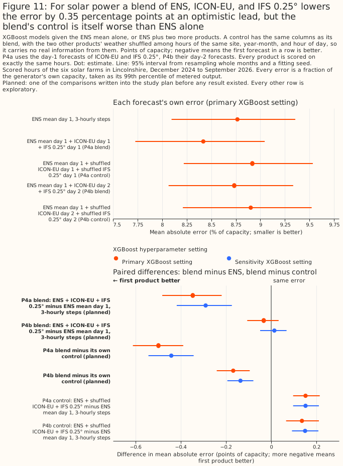
Figure 11: For solar power a blend of ENS, ICON-EU, and IFS 0.25° lowers the error by 0.35 percentage points at an optimistic lead, but the blend's control is itself worse than ENS alone.

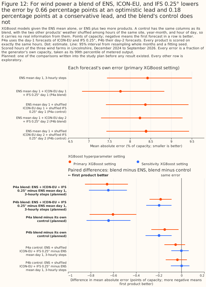
Figure 12: For wind power a blend of ENS, ICON-EU, and IFS 0.25° lowers the error by 0.66 percentage points at an optimistic lead and 0.18 percentage points at a conservative lead, and the blend's control does not.

A second-shuffle refit of the blends on the GPU leaves the wind blend claim in place, and shows that every solar control is worse than ENS alone. Each published blend guard subtracts one shuffled control, and two shuffles of the same AIFS Single weather differ by +0.453 [+0.223, +0.696] points for solar and +0.266 [-0.051, +0.626] points for wind (see the AIFS section). The study therefore refitted P4a and P4b on the published rows and folds on the GPU, with the published shuffle and a second shuffle under another seed, both within generator, year-month, and hour of day. Every contrast in the refit is exploratory. The published CPU numbers stay as published, and the GPU refit sits beside them.

Refit on the GPU, primary setting (points)	Solar P4a	Solar P4b	Wind P4a	Wind P4b
Blend minus ENS day 1	-0.348 [-0.477, -0.222]	-0.029 [-0.097, +0.040]	-0.605 [-0.808, -0.387]	-0.175 [-0.289, -0.076]
Blend minus first control (published shuffle)	-0.495 [-0.596, -0.385]	-0.161 [-0.224, -0.096]	-0.574 [-0.778, -0.354]	-0.169 [-0.272, -0.068]
Blend minus second control (second seed)	-0.437 [-0.560, -0.313]	-0.123 [-0.216, -0.033]	-0.605 [-0.790, -0.405]	-0.182 [-0.273, -0.094]
First control minus ENS day 1	+0.147 [+0.080, +0.215]	+0.133 [+0.059, +0.209]	-0.031 [-0.094, +0.023]	-0.007 [-0.076, +0.054]
Second control minus ENS day 1	+0.088 [+0.025, +0.175]	+0.094 [+0.028, +0.176]	-0.000 [-0.072, +0.065]	+0.007 [-0.070, +0.084]
Seed-to-seed gap: first control minus second	+0.059 [-0.008, +0.125]	+0.039 [-0.021, +0.096]	-0.031 [-0.099, +0.031]	-0.013 [-0.087, +0.055]

The GPU refit's ENS day-1 error is 8.771% [8.096, 9.373] for solar and 8.350% [7.373, 9.364] for wind, and the blends' errors are 8.422% and 8.742% for solar (P4a and P4b) and 7.745% and 8.175% for wind.

The two shuffle seeds agree on every guard, at both settings. The seed-to-seed gap is not statistically significant at the 5% level for either blend or technology at the primary setting, and its interval includes zero at the sensitivity setting too (solar P4a +0.050 [-0.005, +0.099], solar P4b +0.039 [-0.008, +0.084], wind P4a +0.035 [-0.021, +0.097], wind P4b +0.014 [-0.046, +0.077]). The blend minus each control has the same sign and significance at both seeds and both settings. The seed noise that the AIFS null control showed is therefore not visible in these controls.

For wind, the blend claim stands: the blend beats both controls, and neither control is worse than ENS alone. Neither wind control differs significantly from ENS alone at either setting, so each guard can discriminate. P4b, the blend a live service could read, has a lower error than ENS alone on the GPU as well as on the CPU.

For solar, all four controls are significantly worse than ENS alone at the primary setting, so their guards are uninformative for the blend claim, and the verdict stays "may lower the error". The controls are worse than ENS alone by +0.088 to +0.147 points, and the same holds at the sensitivity setting. A blend that beats a control that is itself worse than ENS alone does not show that the added weather carries information. P4b minus ENS alone is -0.029 points [-0.097, +0.040], which includes zero, so the solar blend claim rests on P4a, whose added runs a live service may not be able to read. The refit removes neither limit.

Part of ENS's advantage is ensemble averaging and timing

The gaps between ENS and the other products are partly gaps in ensemble averaging and timing, not only gaps in weather-model quality, and the evidence differs between solar and wind. ENS is averaged over its ensemble members, whereas each Previous Runs product is one run. The study has no contrast that separates ENS's H3-cell average from a Previous Runs product's single grid point. The contrasts below show how much of each gap remains when the ensemble averaging or the hourly timing is removed.

A single ENS control run has a higher error than the ENS mean, and against the control run the wind differences for ICON-EU, ICON-D2, and ICON global are not statistically significant. The ENS control run is one run of the ensemble at ENS's own day-1 lead. The ENS mean minus the control run at day 1 is -0.300 points [-0.447, -0.130] for solar and -0.307 points [-0.440, -0.191] for wind, so averaging the ensemble members lowers the error (exploratory, primary setting only).

Exploratory: day-1 product minus ENS control run (points, primary)	Solar	Wind
UKV	+0.942 [+0.545, +1.377]	+0.463 [+0.151, +0.733]
ICON-D2	+0.802 [+0.432, +1.281]	-0.098 [-0.364, +0.137]
ICON-EU	+0.517 [+0.284, +0.778]	-0.138 [-0.403, +0.100]
ICON global	+0.695 [+0.373, +1.091]	+0.212 [-0.145, +0.632]
IFS 0.25°	-0.264 [-0.498, -0.033]	-0.304 [-0.514, -0.095]
GFS	+1.851 [+1.493, +2.250]	+0.329 [+0.052, +0.584]
GEFS mean	+0.972 [+0.680, +1.269]	+0.551 [+0.274, +0.772]

The control-run contrasts favour the Previous Runs products, because those products have a shorter lead than the control run on most hours. The control run has a lead of 24 + h hours, and the Previous Runs products' leads are shorter on most hours (How the leads are matched). Only GEFS has the control run's exact lead. The table also compares products with different native grids: ICON-EU's is 6.5 km, ICON-D2's is 2.2 km, UKV's is 1.5 km, and the control run's is about 9 km.

For wind, ICON-EU, ICON-D2, and ICON global have no detectable difference from the single ENS control run, and for solar every ICON product still has a higher error. IFS 0.25° has a lower error than the control run for both technologies. UKV has a higher error than the control run for both technologies, and GEFS has a higher error for both. The single-run contrasts are exploratory and use the primary setting only.

Averaging the forecasts over 3 hours or a day shrinks the wind gaps to ENS relative to ENS's own error, and does not shrink the solar gaps (exploratory). Each product's predictions and the measurements are averaged over the block before the error is scored. ENS and GEFS reach the XGBoost model as smoothed 3-hourly fields, so a gap that shrinks as the block lengthens may reflect that smoothing rather than forecast skill. Only GEFS shares ENS's lead.

Exploratory: difference from ENS day 1 (points, primary)	1 hour	3 hours	1 day
Solar, UKV	+1.242 [+0.824, +1.689]	+0.984 [+0.560, +1.425]	+0.945 [+0.453, +1.480]
Solar, ICON-EU	+0.817 [+0.584, +1.069]	+0.655 [+0.416, +0.904]	+0.590 [+0.296, +0.877]
Solar, ICON-D2	+1.102 [+0.704, +1.633]	+0.942 [+0.541, +1.473]	+0.925 [+0.468, +1.451]
Solar, GEFS	+1.272 [+0.937, +1.601]	+1.155 [+0.826, +1.468]	+1.300 [+0.925, +1.673]
Wind, UKV	+0.770 [+0.460, +1.057]	+0.458 [+0.165, +0.731]	+0.303 [-0.119, +0.666]
Wind, ICON-EU	+0.169 [-0.064, +0.384]	+0.031 [-0.194, +0.242]	-0.083 [-0.393, +0.218]
Wind, ICON-D2	+0.209 [-0.015, +0.426]	+0.038 [-0.183, +0.268]	-0.147 [-0.435, +0.128]
Wind, GEFS	+0.858 [+0.598, +1.099]	+0.875 [+0.607, +1.123]	+0.689 [+0.397, +1.006]

Averaging shortens every error, so the table below states each gap as a share of ENS's own error at the same block length (exploratory).

Exploratory: gap as % of ENS's own error at that block length (primary), with 95% interval	1 hour	3 hours	1 day
Solar, ENS's own error (% of capacity)	8.766	6.817	5.830
Solar, UKV	+14.2% [+9.4%, +19.3%]	+14.4% [+8.2%, +20.9%]	+16.2% [+7.8%, +25.4%]
Solar, ICON-EU	+9.3% [+6.7%, +12.2%]	+9.6% [+6.1%, +13.3%]	+10.1% [+5.1%, +15.0%]
Solar, ICON-D2	+12.6% [+8.0%, +18.6%]	+13.8% [+7.9%, +21.6%]	+15.9% [+8.0%, +24.9%]
Solar, GEFS	+14.5% [+10.7%, +18.3%]	+16.9% [+12.1%, +21.5%]	+22.3% [+15.9%, +28.7%]
Wind, ENS's own error (% of capacity)	8.427	7.482	5.233
Wind, UKV	+9.1% [+5.5%, +12.5%]	+6.1% [+2.2%, +9.8%]	+5.8% [-2.3%, +12.7%]
Wind, ICON-EU	+2.0% [-0.8%, +4.6%]	+0.4% [-2.6%, +3.2%]	-1.6% [-7.5%, +4.2%]
Wind, ICON-D2	+2.5% [-0.2%, +5.1%]	+0.5% [-2.4%, +3.6%]	-2.8% [-8.3%, +2.4%]
Wind, GEFS	+10.2% [+7.1%, +13.0%]	+11.7% [+8.1%, +15.0%]	+13.2% [+7.6%, +19.2%]

Each interval is the gap's paired interval divided by ENS's own error at that block length, and the division treats ENS's own error as fixed.

For solar, the gaps shrink in points but not relative to ENS's own error, so the block averages give no support for a timing-noise reading of the solar gaps (exploratory). Averaging over a day cuts ENS's own error from 8.766% to 5.830% of capacity, and every solar gap is statistically significant at every block length. For every product, though, the share's interval at 1 hour overlaps its interval over 1 day, so the study cannot show that any solar share changed with the block length.

For wind, the gaps of the Previous Runs products shrink relative to ENS's own error, which is consistent with timing noise accounting for part of them, and GEFS's gap does not shrink (exploratory). UKV's gap falls from 9.1% of ENS's own error at 1 hour to 5.8% over 1 day, and the 1-day UKV gap is not statistically significant at the 5% level. The hourly gaps of ICON-EU and ICON-D2 already had intervals that include zero, so averaging did not turn a significant ICON gap into a null gap. GEFS's gap is statistically significant at every block length and rises from 10.2% to 13.2% of ENS's own error. The shrinkage for the Previous Runs products does not show whether timing noise or grid-point sampling accounts for more of the wind gap. The share's interval at 1 hour also overlaps its interval over 1 day for every wind product, so the study cannot show that any wind share changed.

Among the other products, IFS 0.25° comes closest to ENS (exploratory)

Among the remaining products, with IFS 0.25° for comparison (all exploratory), only IFS 0.25° avoids the verdict "loses" for solar, and only IFS 0.25° and ICON-D2 avoid the verdict "loses" for wind, as ICON-EU does in its planned wind contrast. The exploratory brackets repeat the planned bracket, at the primary setting only, for every other day and for every other Previous Runs product: Météo-France's AROME and ARPEGE, the HARMONIE-AROME runs of the Danish Meteorological Institute (DMI) and the Royal Netherlands Meteorological Institute (KNMI), GFS, ICON-D2, and ICON global. The table gives the upper-side contrast at day 1: the product minus ENS at day 1. A positive, significant contrast is a verdict of "loses".

Product, day 1 minus ENS day 1 (points, primary)	Solar	Wind
AROME	+1.106 [+0.738, +1.479]	no wind arm
ARPEGE	+1.549 [+1.210, +1.879]	no wind arm
DMI HARMONIE-AROME	+1.084 [+0.748, +1.421]	+0.746 [+0.352, +1.270]
GFS	+2.152 [+1.746, +2.544]	+0.636 [+0.394, +0.856]
ICON-D2	+1.102 [+0.704, +1.633]	+0.209 [-0.015, +0.426] (unresolved)
ICON global	+0.995 [+0.673, +1.418]	+0.519 [+0.193, +0.914]
IFS 0.25°	+0.036 [-0.225, +0.296] (unresolved)	+0.003 [-0.163, +0.186] (unresolved)
KNMI HARMONIE-AROME	+1.330 [+0.857, +1.926]	+0.684 [+0.388, +1.037]

At days 2 and 3, IFS 0.25° stays unresolved against ENS, and ICON-EU at day 2 still loses. For solar, IFS 0.25° minus ENS is -0.132 points [-0.362, +0.092] at day 2 and +0.120 points [-0.108, +0.332] at day 3, both unresolved. For wind the IFS 0.25° contrasts are -0.280 points [-0.470, -0.095] at day 2 and -0.278 points [-0.629, +0.078] at day 3. The wind verdict is unresolved for both days because the lower side of the bracket, the IFS 0.25° error minus ENS's error one day earlier, is positive: +0.857 points [+0.613, +1.123] at day 2 and +1.335 points [+1.049, +1.633] at day 3. ICON-EU day 2 has upper sides of +0.906 points [+0.646, +1.157] for solar and +0.430 points [+0.217, +0.653] for wind, and both verdicts are "loses". The lower side of IFS 0.25° at day 1 for wind is +0.947 points [+0.796, +1.105].

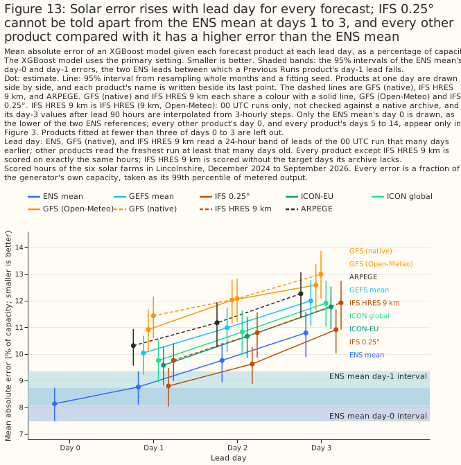
Figure 13: Solar error rises with lead day for every forecast; IFS 0.25° cannot be told apart from the ENS mean at days 1 to 3, and every other product compared with it has a higher error than the ENS mean.

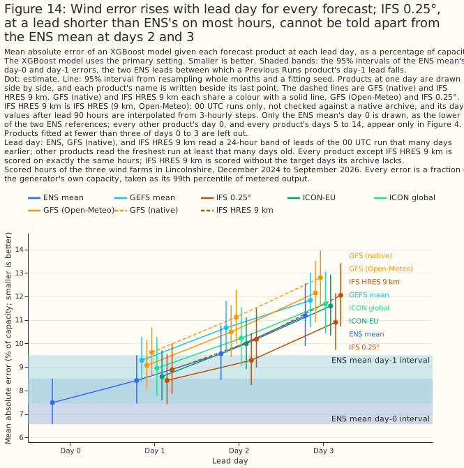
Figure 14: Wind error rises with lead day for every forecast; IFS 0.25°, at a lead shorter than ENS's on most hours, cannot be told apart from the ENS mean at days 2 and 3.

UKV loses to ENS before and after its 2026-01-21 upgrade (exploratory)

UKV loses to ENS both before and after the upgrade of 2026-01-21 (exploratory). Before the upgrade, UKV minus ENS day 1 is +1.056 points [+0.478, +1.674] for solar (22,621 rows in 13 months) and +0.772 points [+0.364, +1.145] for wind (26,923 rows in 13 months). After the upgrade, the differences are +1.577 points [+1.116, +2.103] for solar (12,642 rows in 8 months) and +0.765 points [+0.406, +1.065] for wind (10,484 rows in 8 months). The lower sides are also positive in both eras. For solar the point estimate is larger after the upgrade, but the two intervals overlap ([+0.478, +1.674] before and [+1.116, +2.103] after), so the study does not show that the gap changed. For wind the two intervals overlap almost entirely.

Neither native GFS nor IFS HRES 9 km has an error detectably lower than the ENS mean at any lead day (exploratory)

Native GFS has a higher error than the ENS mean at every lead day from 1 to 10 for both technologies, and at day 0 for solar, and IFS HRES 9 km has a higher error at every lead day fitted. The companion page holds the day-by-day tables, the comparison of native GFS with GFS (Open-Meteo), and the comparison of IFS HRES 9 km with IFS 0.25° and ICON-EU.

AIFS Single has a lower wind error than ENS's control member at day 1, and no solar difference is claimable

On the 16 months of hours that AIFS Single covers (the single and ens row sets are defined in How AIFS is read), AIFS Single has a lower wind error than ENS's control member at day 1 at both XGBoost settings, and the solar difference is not claimable. The contrast is the one AIFS contrast planned before any AIFS fit, and it is the study's deciding contrast for AIFS. Both arms read 6-hourly steps, so the comparison does not favour ENS's finer steps. AIFS Single's day-1 error is 9.402% [8.708, 10.116] of capacity for solar against 9.496% [8.756, 10.281] for the ENS control member, and 8.334% [7.550, 9.167] for wind against 8.916% [7.853, 10.147]. For wind the difference is statistically significant at the 5% level at both settings, and stays significant with a 97.5% interval, and every dropped month keeps the sign (the estimate runs from -0.673 to -0.357 points). The estimate shrinks to -0.207 [-0.414, -0.013] points when both arms lose day of year, and the study did not establish why. For solar every interval includes zero, and the estimate runs from -0.188 to -0.006 points when each month is dropped in turn, so the study makes no solar claim.

Deciding contrast: AIFS Single day 1 minus ENS control member day 1, both on 6-hourly steps (points)	Solar	Wind
Primary setting, 95% interval	-0.094 [-0.426, +0.260]	-0.581 [-1.126, -0.150]
Sensitivity setting, 95% interval	-0.129 [-0.459, +0.222]	-0.501 [-0.912, -0.132]
Primary setting, without day of year in either arm	-0.124 [-0.446, +0.203]	-0.207 [-0.414, -0.013]
Primary setting, 97.5% interval (Bonferroni across solar and wind)	-0.094 [-0.477, +0.311]	-0.581 [-1.233, -0.118]

Against ENS's mean on the same 6-hourly steps, AIFS Single at day 1 is not better, and at day 2 the result differs between solar and wind (exploratory and post hoc). AIFS Single minus the ENS mean at day 1 is +0.148 [-0.043, +0.349] points for solar and -0.182 [-0.514, +0.100] points for wind. At day 2 the difference is -0.268 [-0.459, -0.067] points for solar, and +0.096 [-0.228, +0.367] points for wind. The ENS mean at day 1 has an error of 9.254% [8.573, 9.969] for solar and 8.516% [7.579, 9.569] for wind. The ENS mean on 3-hourly steps has a lower error still (9.010% [8.346, 9.732] and 8.195% [7.248, 9.285]), and the positive control passes: 6-hourly steps raise the ENS mean's error by +0.243 [+0.153, +0.332] points for solar and +0.321 [+0.206, +0.419] points for wind.

Row set single (16 months): each arm's own error (% of capacity, primary)	Solar	Wind
AIFS Single, day 1	9.402% [8.708, 10.116]	8.334% [7.550, 9.167]
AIFS Single, day 2	10.031% [9.229, 10.762]	9.873% [8.600, 11.361]
AIFS Single, day 1, nearest cell	9.386% [8.679, 10.115]	8.320% [7.529, 9.161]
ENS mean, day 1, 6-hourly steps	9.254% [8.573, 9.969]	8.516% [7.579, 9.569]
ENS mean, day 2, 6-hourly steps	10.299% [9.558, 10.988]	9.776% [8.501, 11.202]
ENS control member, day 1, 6-hourly steps	9.496% [8.756, 10.281]	8.916% [7.853, 10.147]
ENS control member, day 2, 6-hourly steps	10.639% [9.771, 11.477]	10.515% [8.935, 12.304]
ENS mean, day 1, 3-hourly steps	9.010% [8.346, 9.732]	8.195% [7.248, 9.285]
IFS 0.25°, day 1, hourly steps	9.073% [8.357, 9.837]	8.141% [7.140, 9.310]
AIFS Single, day 1, shuffled weather	15.582% [14.438, 16.808]	18.912% [16.399, 21.512]

Row set single: exploratory, post hoc contrasts (points, primary)	Solar	Wind
AIFS Single day 1 − ENS mean day 1 (6-hourly steps)	+0.148 [-0.043, +0.349]	-0.182 [-0.514, +0.100]
AIFS Single day 2 − ENS control member day 2 (6-hourly steps)	-0.608 [-0.925, -0.302]	-0.643 [-1.195, -0.188]
AIFS Single day 2 − ENS mean day 2 (6-hourly steps)	-0.268 [-0.459, -0.067]	+0.096 [-0.228, +0.367]
AIFS Single day 1 − IFS 0.25° day 1 (hourly steps, one-sided reference)	+0.329 [+0.088, +0.583]	+0.194 [-0.284, +0.594]
AIFS Single day 1 − AIFS Single day 1, nearest cell	+0.016 [-0.021, +0.050]	+0.014 [-0.028, +0.056]
ENS mean 6-hourly − ENS mean 3-hourly, day 1 (positive control)	+0.243 [+0.153, +0.332]	+0.321 [+0.206, +0.419]
AIFS Single day 1 − the same arm with shuffled weather	-6.180 [-7.100, -5.387]	-10.578 [-12.609, -8.648]
Two shuffles of AIFS Single's weather, one minus the other (null)	+0.453 [+0.223, +0.696]	+0.266 [-0.051, +0.626]

Row set single: pairs near the 5% line, sensitivity setting (points)	Solar	Wind
AIFS Single day 1 − ENS mean day 1 (6-hourly steps)	+0.115 [-0.072, +0.318]	-0.134 [-0.375, +0.105]
AIFS Single day 2 − ENS control member day 2 (6-hourly steps)	not fitted	-0.538 [-1.007, -0.155]
AIFS Single day 2 − ENS mean day 2 (6-hourly steps)	-0.242 [-0.445, -0.016]	not fitted
AIFS Single day 1 − IFS 0.25° day 1 (hourly steps, one-sided reference)	+0.284 [+0.035, +0.549]	not fitted
Two shuffles of AIFS Single's weather, one minus the other (null)	not fitted	+0.422 [+0.137, +0.833]

Reading AIFS Single from the nearest cell instead of the cell average changes nothing detectable, and shuffling AIFS Single's weather raises the error by several points. The nearest-cell difference is +0.016 [-0.021, +0.050] points for solar and +0.014 [-0.028, +0.056] points for wind. AIFS Single minus the arm given AIFS Single's weather shuffled among hours of the same generator, year-month, and UTC hour is -6.180 [-7.100, -5.387] points for solar and -10.578 [-12.609, -8.648] points for wind, so AIFS Single's weather carries information beyond the calendar and the sun's position. Two different shuffles of the same weather differ by +0.453 [+0.223, +0.696] points for solar and +0.266 [-0.051, +0.626] points for wind (+0.422 [+0.137, +0.833] points at the sensitivity setting), so this null control fails: two arms that carry the same information differ significantly at the 5% level. The month-and-seed intervals therefore do not cover the difference between one shuffle and another, and any contrast against a shuffled arm, including the blend guards in the blend section, may carry noise of that size which its interval does not show. The deciding AIFS contrast involves no shuffled arm.

The sign of the AIFS Single minus ENS mean difference changes between version eras, and each era covers different months as well as a different version (exploratory). The eras hold 5, 7, and 4 months, and the report prints an interval only for an era of 6 months or more. The version change, the season, and IFS Cycle 50r1 (which began with AIFS Single v2 on 2026-05-12) cannot be separated.

Row set single: AIFS Single day 1 − ENS mean day 1 (6-hourly steps) by version era (points, primary; months with the era's sign)	Solar	Wind
Era 0, AIFS Single v1.0 (5 months)	+0.103 (3 of 5)	-0.092 (3 of 5)
Era 1, AIFS Single v1.1 (7 months)	+0.346 [-0.073, +0.699] (4 of 7)	-0.455 [-1.071, +0.062] (5 of 7)
Era 2, AIFS Single v2 (4 months)	-0.033 (2 of 4)	+0.245 (3 of 4)

The AIFS ENS contrasts are descriptive only. About 84% of the scored (generator, fold, calendar month) cells of the 11-month row set have no training row of their calendar month, so an XGBoost model scores most of its months in a season it has not seen. The tables give the absolute error beside each contrast, and none of these results is a claim.

Row set ens (11 months): each arm's own error (% of capacity, primary)	Solar	Wind
AIFS ENS mean, day 1	9.243% [8.280, 10.023]	8.949% [7.842, 10.049]
AIFS ENS mean, day 2	9.986% [8.781, 11.029]	10.296% [8.811, 11.798]
AIFS Single, day 1	9.337% [8.272, 10.205]	9.003% [7.957, 10.010]
ENS mean, day 1, 6-hourly steps	9.233% [8.345, 9.941]	9.205% [7.853, 10.537]
ENS mean, day 2, 6-hourly steps	10.118% [8.977, 11.128]	10.796% [9.057, 12.556]

Row set ens: descriptive contrasts (points, primary)	Solar	Wind
AIFS ENS mean day 1 − ENS mean day 1 (6-hourly steps)	+0.010 [-0.166, +0.212]	-0.257 [-0.610, +0.086]
AIFS ENS mean day 2 − ENS mean day 2 (6-hourly steps)	-0.133 [-0.388, +0.100]	-0.500 [-0.931, -0.110]
AIFS ENS mean day 1 − AIFS Single day 1	-0.095 [-0.294, +0.109]	-0.055 [-0.290, +0.181]
AIFS ENS mean day 2 − AIFS Single day 2	+0.120 [-0.209, +0.415]	-0.644 [-1.277, -0.196]

Row set ens: pairs near the 5% line, sensitivity setting (points, descriptive)	Solar	Wind
AIFS ENS mean day 1 − ENS mean day 1 (6-hourly steps)	not fitted	-0.107 [-0.367, +0.130]
AIFS ENS mean day 2 − ENS mean day 2 (6-hourly steps)	not fitted	-0.265 [-0.576, +0.009]
AIFS ENS mean day 2 − AIFS Single day 2	not fitted	-0.478 [-0.741, -0.223]

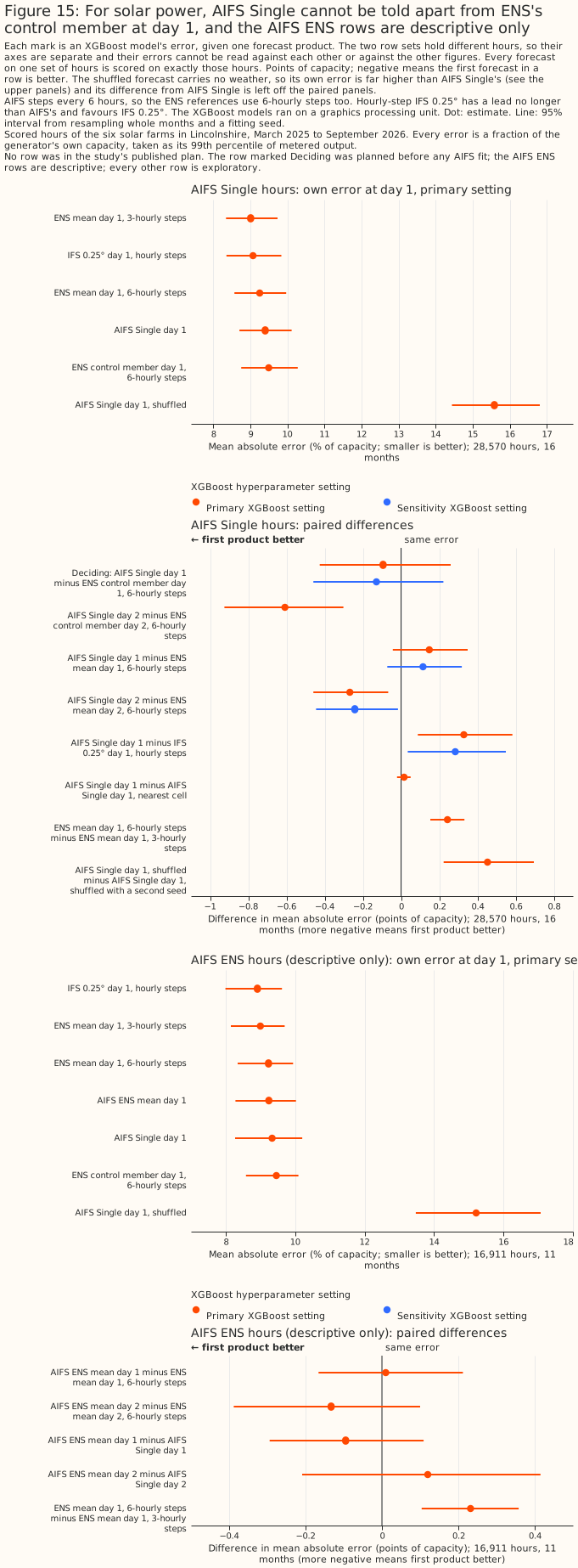
Figure 15: For solar power, AIFS Single cannot be told apart from ENS's control member at day 1, and the AIFS ENS rows are descriptive only.

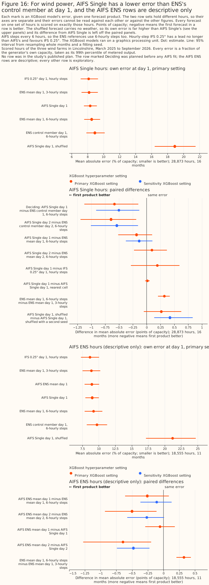
Figure 16: For wind power, AIFS Single has a lower error than ENS's control member at day 1, and the AIFS ENS rows are descriptive only.

At day 7 a blend of ENS and AIFS Single lowers the solar error, and at day 14 no forecast has skill to compare

At day 7, giving an XGBoost model both ENS's mean and AIFS Single lowers the solar error, and the wind difference is not claimable. At day 14, neither technology has any skill to compare. This section is exploratory, except the four deciding contrasts per technology (H7, H14, B7, and B14) that How AIFS is read names. Every number is at the primary setting unless a row says otherwise. The rows are the single row set, 6 solar farms and 3 wind farms, 16 months, and the AIFS Single versions those months hold. The survey page says that AIFS has not been shown to improve faster than the physics-based IFS and that each AIFS version should be scored separately, and this section treats AIFS Single as a forecast that has a lower or higher error, never as one that has improved.

Row set single: each arm's own error (% of capacity, primary)	Solar day 7	Solar day 14	Wind day 7	Wind day 14
AIFS Single	14.198% [13.023, 15.531]	15.287% [14.187, 16.562]	17.355% [15.186, 19.546]	19.426% [16.763, 22.161]
ENS control member	14.638% [13.572, 15.812]	15.321% [14.164, 16.604]	17.909% [16.009, 19.796]	18.892% [16.472, 21.526]
ENS mean	14.297% [13.188, 15.561]	15.207% [14.114, 16.446]	16.555% [14.754, 18.423]	18.599% [16.262, 21.033]
Blend of ENS mean and AIFS Single	13.901% [12.753, 15.236]	15.236% [14.154, 16.465]	16.281% [14.401, 18.155]	18.901% [16.465, 21.376]
Blend with AIFS Single's weather shuffled	14.338% [13.257, 15.604]	15.311% [14.215, 16.565]	16.605% [14.754, 18.488]	18.522% [16.221, 20.882]
AIFS Single with its weather shuffled (first seed)	15.351% [14.218, 16.651]	15.441% [14.287, 16.738]	18.966% [16.390, 21.512]	18.856% [16.247, 21.508]
IFS 0.25° (hourly steps)	14.929% [13.835, 16.171]	not fitted	17.966% [15.752, 20.141]	not fitted
IFS HRES 9 km	14.701% [13.626, 15.822]	not fitted	17.858% [15.993, 19.701]	not fitted

The table's rows differ by day in the rows scored (28,208 solar and 28,419 wind rows at day 7, 27,449 and 27,440 at day 14). IFS HRES 9 km lacks some target days, so on the 28,041 solar rows and 28,294 wind rows it has, its error is 14.674% [13.606, 15.813] and 17.839% [15.960, 19.695]. IFS 0.25° and IFS HRES 9 km are not fitted at day 14 (their archives stop at day 7 and day 10).

For solar power at day 7, the blend of ENS's mean and AIFS Single lowers the error against ENS's mean alone, and the shuffled control shows the gain comes from AIFS Single's weather (B7, deciding). The blend's error is 13.901% against 14.297% for ENS's mean alone, a difference of -0.396 points [-0.578, -0.201]. The difference is -0.258 points [-0.432, -0.077] at the sensitivity setting, and -0.396 points [-0.632, -0.118] at the 99.375% Bonferroni level. With each month dropped in turn the estimate runs from -0.454 to -0.359 points, so no month reverses the sign. The guard, the blend minus the blend given shuffled AIFS Single weather, is -0.437 points [-0.674, -0.169] at the primary setting and -0.342 points [-0.547, -0.128] at the sensitivity setting. The shuffled control is not significantly worse than ENS's mean alone (+0.041 points [-0.126, +0.198]), so the guard can discriminate. The verdict is that the blend lowers the error at day 7 for these six solar farms. The gain is 0.396 points of capacity, about 2.8% of ENS's mean's own error.

For wind power at day 7, the blend's gain over ENS's mean is not claimable. The difference is -0.274 points [-0.586, +0.064] at the primary setting, which includes zero, and -0.361 points [-0.529, -0.183] at the sensitivity setting, which does not. The guard is -0.325 points [-0.667, -0.007] at the primary setting and -0.414 points [-0.621, -0.199] at the sensitivity setting. The verdict is no detectable difference, and a gain as large as 0.586 points is not excluded. Every dropped month keeps the sign of the estimate.

AIFS Single alone has a significantly lower solar error than ENS's control member at day 7 at the primary setting only, and neither technology's difference is claimable (H7, deciding). For solar the difference is -0.440 points [-0.759, -0.074] at the primary setting and -0.412 points [-0.784, +0.072] at the sensitivity setting, and without day of year in either arm it is -0.257 points [-0.567, +0.073]. The primary interval is statistically significant at the 5% level and the other two are not, so H7 fails the rule. For wind the difference is -0.554 points [-1.234, +0.195], and -0.431 points [-0.969, +0.091] at the sensitivity setting. Against ENS's mean, AIFS Single at day 7 does not have a significantly lower error for either technology (exploratory): -0.099 points [-0.419, +0.276] for solar, and +0.800 points [+0.015, +1.586] for wind, where AIFS Single has the higher error. AIFS Single and the ENS mean are close for solar, and the ENS control member is the noisier forecast (positive control, control minus ENS mean: +0.341 points [+0.061, +0.619] for solar and +1.354 points [+0.859, +1.949] for wind). The solar H7 result is therefore consistent with AIFS Single being smoother than the control member, and the page does not describe it as a better weather forecast. AIFS Single's day-7 solar radiation has a standard deviation of 199.0 W/m², against 213.7 for the control member and 191.5 for the ENS mean.

AIFS Single has a lower day-7 error than IFS 0.25° for both technologies, and than IFS HRES 9 km for solar only at one setting (exploratory). The comparison with IFS 0.25° is one-sided, because IFS 0.25° reads hourly steps and a shorter lead, both of which favour IFS 0.25°. AIFS Single minus IFS 0.25° is -0.731 points [-1.112, -0.341] for solar (14.198% against 14.929%) and -0.611 points [-1.019, -0.227] for wind (17.355% against 17.966%). On the rows IFS HRES 9 km has, AIFS Single minus IFS HRES 9 km is -0.441 points [-0.784, -0.017] for solar (14.232% against 14.674%) and -0.442 points [-1.080, +0.202] for wind (17.397% against 17.839%). The solar difference against IFS HRES 9 km is -0.447 points [-0.841, +0.046] at the sensitivity setting, so it lies near the 5% line. AIFS Single's weather carries information at day 7: shuffling it raises the error by 1.153 points [+0.706, +1.574] for solar and 1.610 points [+0.835, +2.511] for wind.

At day 14, neither AIFS Single nor the ENS control member has an error below the shuffled arms, so there is no skill to compare, for solar or for wind. Under the reading rule, ENS's control member minus AIFS Single with shuffled weather is -0.120 points [-0.403, +0.154] and +0.078 points [-0.160, +0.339] for solar (two shuffle seeds), and +0.035 points [-0.545, +0.570] and +0.055 points [-0.701, +0.736] for wind. The same contrasts for AIFS Single itself include zero too. H14 and B14 are therefore not read. Their intervals are for completeness: for solar, AIFS Single minus the control member is -0.035 points [-0.305, +0.216] and the blend minus ENS's mean is +0.029 points [-0.239, +0.267]; for wind, +0.534 points [-0.334, +1.535] and +0.302 points [+0.015, +0.644]. The wind blend has a higher error than ENS's mean at the primary setting, and not at the sensitivity setting (+0.115 points [-0.075, +0.336]), so the wind blend at day 14 is unresolved.

The AIFS-versus-IFS test at day 14 rests on the ENS control member, and not on IFS HRES. The ENS control member is the IFS model run as an ensemble with perturbed initial conditions, so a day-14 contrast with the control member says nothing about IFS HRES 9 km, which the study fits no further than day 7.

The gap between AIFS Single and the ENS control member moves against AIFS Single from day 7 to day 14 (exploratory and post hoc). On the day-14 rows, the difference in that gap is +0.468 points [+0.047, +0.818] for solar and +1.136 points [-0.023, +2.359] for wind. On those rows the solar gap is -0.503 points at day 7 (14.098% against 14.601%) and -0.034 points at day 14 (15.287% against 15.321%). The wind gap is -0.601 points at day 7 (17.343% against 17.944%) and +0.534 points at day 14 (19.426% against 18.892%).

At days 1 and 2 the blend's gain over ENS's mean varies by technology and day (exploratory and post hoc). Solar: the blend minus ENS's mean is -0.044 points [-0.162, +0.073] at day 1 and -0.325 points [-0.479, -0.181] at day 2, with guards of -0.116 points [-0.241, +0.009] and -0.385 points [-0.512, -0.263]. Wind: -0.305 points [-0.603, -0.099] at day 1 and -0.211 points [-0.383, -0.049] at day 2, with guards of -0.292 points [-0.504, -0.123] and -0.140 points [-0.347, +0.075]. At day 1 the solar guard's sensitivity-setting interval is -0.130 points [-0.242, -0.021]. Blending AIFS ENS's mean with ENS's mean is descriptive only, for the fold-coverage reason above.

AIFS ENS's mean is close to ENS's mean at days 7 and 14 too, for both technologies (descriptive only). For solar, AIFS ENS's mean minus ENS's mean is +0.066 points [-0.193, +0.360] at day 7 (14.208% against 14.142%) and -0.287 points [-0.701, +0.097] at day 14 (15.083% against 15.370%). For wind, it is +0.341 points [-0.746, +1.630] at day 7 (18.104% against 17.763%) and +0.263 points [-1.316, +1.968] at day 14 (20.982% against 20.719%). These four contrasts carry the same fold-coverage limitation as the day-1 and day-2 AIFS ENS rows above, and none is a claim.

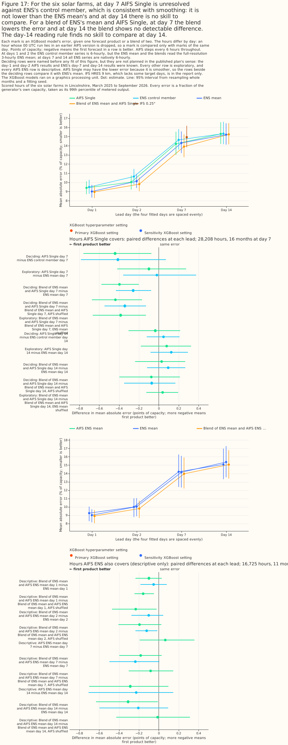
Figure 17: For the six solar farms, at day 7 AIFS Single is unresolved against ENS's control member, which is consistent with smoothing: it is not lower than the ENS mean's and at day 14 there is no skill to compare. For a blend of ENS's mean and AIFS Single, at day 7 the blend lowers the error and at day 14 the blend shows no detectable difference. The day-14 reading rule finds no skill to compare at day 14.

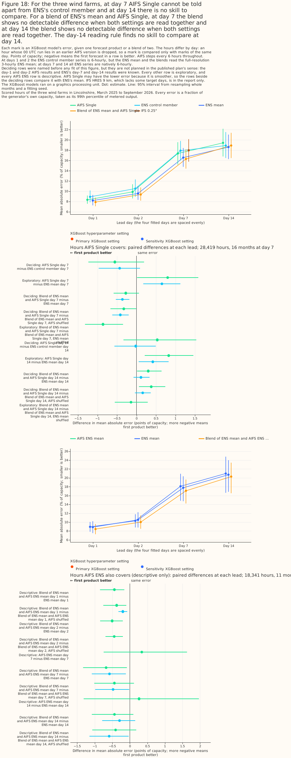
Figure 18: For the three wind farms, at day 7 AIFS Single cannot be told apart from ENS's control member and at day 14 there is no skill to compare. For a blend of ENS's mean and AIFS Single, at day 7 the blend shows no detectable difference when both settings are read together and at day 14 the blend shows no detectable difference when both settings are read together. The day-14 reading rule finds no skill to compare at day 14.

WN3's mean has a lower point error than ENS's mean at days 1 and 2, and at days 7 and 14 no WN3 difference is claimable

In the pooled rows (February to September 2026), the error of an XGBoost model given WN3's mean is lower than the error given ENS's mean at days 1 and 2 for solar and wind, and at days 7 and 14 every pooled interval spans 0. The July to September rows are the check for overlap with WN3's training data. Their intervals resample only 3 months, fewer than the study's minimum of 6, so they give the range of the months and are indicative only. The lead July to September difference, solar day 2 at -0.318 points [-0.584, -0.064], is a point estimate: the two shuffled-weather arms differ by +0.321 [+0.033, +0.616] in the same cell. The wind contrast is against the matched ENS mean-vector reference (How WeatherNext 3 is read), and every wind number below is against that reference unless stated. Every difference is descriptive, because each calendar month occurs in one year only. Each difference is WN3's error minus the reference's, in points of capacity, so a negative difference means WN3 has the lower error.

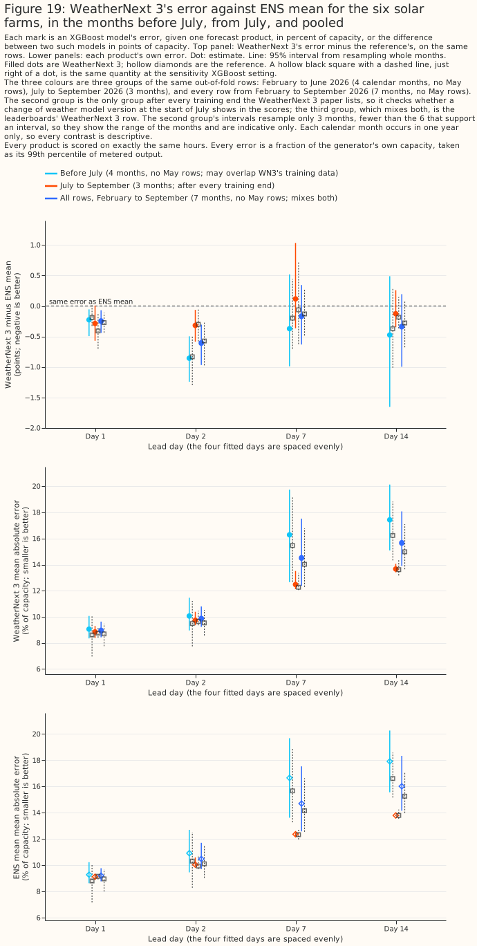
Figure 19: For the six solar farms, WN3's mean has a lower error than ENS's mean at day 1 and day 2 in all three groups of rows, but February to June may overlap WeatherNext 3's training data. The July to September difference at day 2 is -0.318 points [-0.584, -0.064], but that interval resamples only 3 months and the two shuffled-weather arms differ by +0.321 [+0.033, +0.616] in the same cell, so read it as a point estimate. At day 7 and day 14 the intervals span 0 in every group. At day 14 the July to September interval is narrow because the 3 months resembled one another, not because the difference is known precisely, and at day 14 the second-seed shuffled arm has the lower error. Hollow squares are the sensitivity setting.

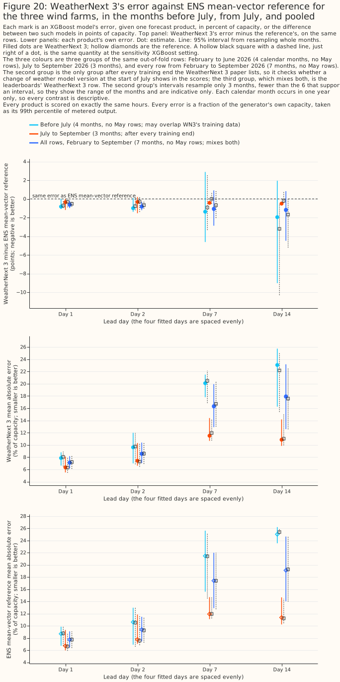
Figure 20: For the three wind farms, WN3's mean has a lower error than ENS's mean-vector reference at day 1 in July to September (-0.358 points [-1.185, -0.002]): the upper bound is -0.002, and at the sensitivity setting the interval is [-0.898, +0.032], which spans 0. February to June may overlap WeatherNext 3's training data. At day 2 the July to September interval spans 0. At day 7 and day 14 the July to September intervals exclude 0 at the primary setting and span 0 at the sensitivity setting. At day 7, WN3's error (11.512%) equals its two shuffled-weather arms' (11.517% and 11.511%), and those arms beat the mean-vector reference (11.926%), so the day-7 contrast measures the reference doing worse than no weather, not WN3 skill. The July to September intervals resample only 3 months, so they are indicative only. Hollow squares are the sensitivity setting.

The three groups agree in sign at every day and technology except solar day 7 in July to September, and the pooled group is the one the leaderboards draw. What is known about WN3's lookahead defines the three groups. The tables give each group's error and difference, at the primary setting, with 95% intervals from resampling whole months. The pooled interval is the only interval of the three that rests on the study's minimum of 6 months. The July to September group is the check for overlap with training data.

Solar power (% of capacity)	In-sample WN3	In-sample ENS mean	July to September WN3	July to September ENS mean	Pooled WN3	Pooled ENS mean
Day 1	9.055%	9.281%	8.841%	9.127%	8.964%	9.208%
Day 2	10.063%	10.919%	9.731%	10.049%	9.879%	10.482%
Day 7	16.284%	16.656%	12.476%	12.359%	14.533%	14.697%
Day 14	17.437%	17.912%	13.669%	13.796%	15.679%	16.014%

Solar power: WN3 minus ENS mean (points)	In-sample	July to September	Pooled
Day 1	-0.226 [-0.494, -0.056]	-0.286 [-0.570, +0.007]	-0.243 [-0.440, -0.069]
Day 2	-0.856 [-1.241, -0.496]	-0.318 [-0.584, -0.064]	-0.603 [-0.966, -0.306]
Day 7	-0.371 [-0.988, +0.518]	+0.117 [-0.365, +1.034]	-0.165 [-0.630, +0.343]
Day 14	-0.475 [-1.654, +0.489]	-0.127 [-0.347, +0.258]	-0.334 [-0.996, +0.194]

Wind power (% of capacity)	In-sample WN3	In-sample ENS reference	July to September WN3	July to September ENS reference	Pooled WN3	Pooled ENS reference
Day 1	7.861%	8.683%	6.348%	6.706%	7.129%	7.730%
Day 2	9.615%	10.606%	7.429%	7.758%	8.580%	9.381%
Day 7	20.093%	21.462%	11.512%	11.926%	16.345%	17.395%
Day 14	23.065%	25.014%	10.861%	11.359%	17.939%	19.098%

Wind power: WN3 minus ENS mean-vector reference (points)	In-sample	July to September	Pooled
Day 1	-0.821 [-1.089, +0.010]	-0.358 [-1.185, -0.002]	-0.601 [-0.979, -0.192]
Day 2	-0.991 [-1.378, +0.105]	-0.329 [-1.528, +0.219]	-0.801 [-1.206, -0.321]
Day 7	-1.369 [-4.618, +2.891]	-0.413 [-0.501, -0.302]	-1.050 [-2.870, +0.917]
Day 14	-1.949 [-9.023, +1.946]	-0.498 [-0.609, -0.359]	-1.159 [-4.480, +0.829]

Wind power, July to September: WN3 minus ENS mean speed (points)	Difference
Day 1	-0.468 [-1.175, -0.099]
Day 2	-0.382 [-1.388, +0.129]
Day 7	-0.050 [-2.213, +0.849]
Day 14	-0.070 [-0.248, +0.519]

At days 7 and 14, the mean-vector reference has a higher error than ENS's mean speed, in July to September, by 0.36 and 0.43 points, so the wind contrasts against the reference at those days partly measure the reference's definition. Against ENS's mean speed, WN3's differences at days 7 and 14 are -0.050 and -0.070 points, and both intervals span 0.

Absolute skill falls steeply with lead, and a gap of a few tenths of a point sits beside errors of 6 to 25% of capacity. At solar day 1 in July to September, WN3's error is 8.841% and ENS's is 9.127%, a gap of 3% of ENS's error. The months before July have errors 1.3 to 2.2 times those of July to September at days 7 and 14, for WN3 and ENS alike, so a difference between the groups' errors is not evidence about WN3's training data.

The negative control shows that WN3's weather carries the skill at days 1 and 2 for both technologies and at day 7 for solar, and carries none detectable at solar day 14 or wind day 7 in July to September. In the control, WN3's weather is shuffled within farm, year-month, and hour of day, under two seeds. At day 1 and day 2, WN3's error minus the shuffled arm's is between -3.4 and -9.8 points for solar and between -4.6 and -17.6 points for wind, in every group, with intervals that exclude 0. At solar day 7 the July to September differences are -1.124 [-1.953, -0.317] and -0.759 [-1.443, -0.320]. At solar day 14, the July to September differences are +0.096 [-0.054, +0.442] and +0.568 [+0.218, +0.781]. At wind day 7 the July to September differences are -0.005 [-0.154, +0.113] and +0.002 [-0.297, +0.273]. At solar day 14 the XGBoost model given the second-seed shuffled weather has the lower error, and at wind day 7 the shuffled arms' error (11.517% and 11.511%) equals WN3's (11.512%) and beats the mean-vector reference's (11.926%). So WN3's mean adds no detectable skill at those two cells, and the wind day-7 contrast of -0.413 points measures the reference doing worse than no weather. The wind day-14 July to September differences, -0.526 [-0.711, -0.314] and -0.405 [-1.010, -0.177], favour the real weather, on 3 months. The two shuffle seeds also differ from each other: the interval of their difference excludes 0 in 5 of the 24 cells of technology, day, and group, and the largest such difference is -2.240 points [-7.471, -0.196], for wind day 2 in the months before July. Shuffling noise is therefore not negligible next to the differences read here. In the pooled rows, no failure of the control is detectable at solar day 14 (+0.124 [-0.600, +0.598]) or at wind day 14 (-0.402 [-1.603, +0.369]), because both intervals span 0.

The sensitivity setting removes the exclusion of 0 from three July to September wind contrasts, at days 1, 7, and 14, and moves the solar day-1 interval off 0. The sensitivity refits fire on contrasts whose interval lies near the 5% line. In July to September, at solar day 1 the difference is -0.409 [-0.700, -0.122] at the sensitivity setting, against -0.286 [-0.570, +0.007] at the primary setting, and at solar day 2 it is -0.300 [-0.579, -0.035]. At wind day 1 the matched contrast is -0.358 [-1.185, -0.002] at the primary setting and -0.303 [-0.898, +0.032] at the sensitivity setting. At wind day 7 the difference is -0.413 [-0.501, -0.302] at the primary setting and +0.011 [-0.536, +0.726] at the sensitivity setting, so the wind day-7 difference depends on the XGBoost setting and is not claimable. At wind day 14 the sensitivity setting gives -0.201 [-0.436, +0.735], against -0.498 [-0.609, -0.359] at the primary setting, so the wind day-14 difference depends on the XGBoost setting too.

The number of rows in each group, and the rows in neither group, are in the report. The months before July hold 6,335 rows for solar and 5,415 for wind at every lead day. The July to September group holds 5,069, 4,995, 4,602, and 4,129 solar rows at days 1, 2, 7, and 14, and 4,773, 4,701, 4,349, and 3,863 wind rows. The pooled group holds 11,479 solar rows and 10,260 wind rows at every day. The rows in neither group are those whose valid month is after June but whose 00 UTC run was issued on or before 30 June: 75, 149, 542, and 1,015 rows for solar at days 1, 2, 7, and 14, and 72, 144, 496, and 982 for wind. In each cell, the two groups' rows plus the rows in neither group sum to the pooled rows. Across the 42 solar and 21 wind (farm, fold, calendar month) cells, none has a training row of its own calendar month. No loss in any saved file is NaN, and the only nulls are the continuous ranked probability scores that a single-valued arm does not have.

WN3 and AIFS at days 0, 3, 4, and 10 (exploratory)

In the pooled rows, WN3's mean has a lower error than ENS's mean at days 3 and 4 for solar and wind, every AIFS point error is lower than ENS's mean at days 3 and 4, and at day 0 the AIFS point errors are higher. At day 10 the AIFS sign changes with the row set and the technology, and WN3's wind error is higher than ENS's in the pooled rows. No AIFS difference is claimed, because the fits give no paired interval. The WN3 differences are against a same-rows ENS mean, and the months before July may overlap WN3's training data. The companion page holds the tables for the three row groups.

Discussion: what to use

Each recommendation below is about a product as this study reads it, and rests on an XGBoost model fitted at nine generators in one area. Each paragraph gives the size of the effect beside ENS's own error, and says whether the live lead, which the study did not measure, would strengthen or weaken the verdict. A live service reads ENS at 09:00 UTC. The Previous Runs day-1 lead of UKV, ICON-EU, and IFS 0.25° is probably shorter than the lead a 09:00 UTC service would get from those products, so the live lead would probably make those products look worse than this study does.

For solar, keep the ECMWF ENS ensemble mean as the day-ahead weather input. UKV and ICON-EU lose to ENS at a matched lead at both settings (P1a and P2a, planned; solar results). Their gaps are +14.2% and +9.3% of ENS's own day-1 error (exploratory shares). UKV's solar radiation is also the study's own reconstruction from two snapshots. What would change the recommendation: a weather product that beats ENS's day-0 error, which no Previous Runs product did (the closest Previous Runs product, IFS 0.25°, is +0.666 points [+0.462, +0.852] behind, exploratory).

For solar, adding ICON-EU and IFS 0.25° to ENS shows no detectable gain at the conservative lead, so the study gives no reason to ingest a second weather model. The contrast that decides the blend verdict, P4b (planned), includes zero at both settings (blend results), and is -0.4% [-1.2%, +0.4%] of ENS's own error (exploratory share). A gain as large as 0.106 points is therefore not excluded, and neither is a loss as large as 0.068 points. Scored on daily means, P4b is -0.097 points [-0.190, -0.016] (exploratory), so a small gain in daily solar energy is possible even though no hourly gain was detected. The optimistic contrast, P4a (planned), shows a gain, but the P4a permutation guard is uninformative and P4a's IFS 0.25° value can come from a run newer than ENS's 00 UTC run. The study did not test how the live lead would move P4b, so the effect of the live lead on this verdict is unknown. What would change the recommendation: a test that separates a second weather model from a newer ECMWF run, such as a solar blend given ICON-EU alone. The blends page fits that blend: at the conservative lead it shows no detectable solar gain at day 1 or day 2.

For solar, the free GEFS ensemble is not a substitute for ENS. At the same lead, an XGBoost model given GEFS's mean has a higher error than an XGBoost model given ENS's mean at both settings (P3, planned; solar results), by +14.5% of ENS's own error (exploratory share). GEFS's own error, 10.039% of capacity, is still well below climatology's 14.458%, so GEFS carries real information. GEFS and ENS have the same lead, so the live lead does not change this verdict.

IFS 0.25° is the closest to ENS of the individual products tested, but the study does not show that IFS 0.25° would match ENS in a live service. IFS 0.25° day 1 cannot be told apart from ENS day 1 for solar or wind (exploratory). IFS 0.25°'s Previous Runs lead is shorter than ENS's on most hours, and its day-1 value can come from a 12 or 18 UTC run published after the 09:00 UTC issue time, so both comparisons favour IFS 0.25°.

For wind, keep ENS and do not use UKV. UKV loses to ENS at a matched lead at both settings (P1a, planned; wind results). On an ENS day-1 error of 8.427% of capacity, the gap is +9.1% of ENS's own error (exploratory share). The study did not test the Met Office's ensemble, the Met Office Global and Regional Ensemble Prediction System for the UK (MOGREPS-UK), so this finding is about UKV as one deterministic run and not about the Met Office's forecasts as a whole. The loss is the same before and after UKV's 2026-01-21 upgrade (exploratory). The gap also shrinks when the forecasts and measurements are averaged over whole days, to +0.303 points [-0.119, +0.666], which is no longer statistically significant at the 5% level (exploratory). What would change the recommendation: a comparison that reads UKV at ENS's exact lead, which the Previous Runs archive cannot supply and Open-Meteo's Single Runs archive might.

For wind, ICON-EU is unresolved against ENS, so the study gives no reason to swap ENS for ICON-EU. The upper side of the bracket (P2a, planned) includes zero and the lower side (P2b) is well above zero (wind results), so ICON-EU sits between ENS's day-0 and day-1 errors. The upper end of the P2a interval means that ICON-EU could be up to 0.384 points worse than ENS, which is 4.6% of ENS's own error of 8.427% (exploratory share). On the night hours where the two leads are exactly equal, 00 to 05 UTC, ENS wins (exploratory). Against a single ENS control run, which has no ensemble averaging, ICON-EU cannot be separated from ENS (exploratory). ICON-EU's Previous Runs day-1 lead is shorter than the control run's lead on most hours of the day, so the control-run comparison favours ICON-EU. ICON-EU's Previous Runs day-1 lead is also probably shorter than the lead a 09:00 UTC service would get. The unmeasured live lead would therefore probably move ICON-EU towards a "loses" verdict, and would strengthen the case for keeping ENS.

For wind, adding ICON-EU and IFS 0.25° to ENS is the one planned contrast against ENS alone that shows a gain at the conservative lead, and the gain is about 0.2 points of capacity. The contrast that decides the blend verdict, P4b (planned), is -0.184 points [-0.282, -0.087] at the primary setting, on an ENS day-1 error of 8.427% of capacity, which is -2.2% [-3.3%, -1.0%] of ENS's own error (exploratory share). The guard is negative and the controls are not significantly worse than ENS alone at both settings (blend results), so the gain comes from the weather of ICON-EU and IFS 0.25° rather than from extra columns. The gain is not the same at every generator: at W1 the P4b interval reaches zero, and each per-generator interval covers month-to-month weather and the fitting seed, not differences between generators (exploratory). The study did not test how the live lead would move P4b, so the effect of the live lead on this verdict is unknown.

A service that ingests one added product would probably get most of the wind gain from ICON-EU (exploratory and post hoc). ICON-EU at day 2 alone, added to ENS, gives -0.169 points [-0.250, -0.090], which is not statistically distinguishable from P4b. Against P4b, ENS plus ICON-EU alone is +0.015 points [-0.033, +0.065], so it could be up to 0.065 points worse than P4b. What would change the recommendation: a different result at more wind generators than the three tested here.

ICON-D2 read at its freshest run has the lowest error of any forecast fitted, but that skill does not carry to day-ahead use (exploratory). A value from a run that started 0 to 3 hours before the hour is not available to a service issuing at 09:00 UTC for the rest of the day. At day 1 ICON-D2 is mid-ranking (Figures 3 and 4), and ICON-D2's domain does not cover all of Great Britain.

Beyond day 3, keep the ENS mean, and do not treat a day-10 or day-14 forecast as skilled beyond climatology at these farms. At days 5 to 10, every product fitted has a higher error than the ENS mean in the point estimates. At day 14, GEFS, native GFS, and the ENS control member have point estimates within 0.2 points of the ENS mean's for solar, and none of them can be told apart from the ENS mean. The ENS mean's error is lower than climatology's at day 7 and cannot be told apart from climatology's at day 10 or day 14 (Error and lead). What would change the recommendation: a test at more generators, or over more months, than these nine farms and 21 months provide. Every lead-day result is exploratory and fitted at the primary setting only.

For day-ahead use, IFS HRES 9 km and native GFS give no reason to replace the ENS mean. Native GFS has a higher error than the ENS mean at equal lead from day 1 to day 10, and IFS HRES 9 km has a higher error at every lead day fitted (native GFS and IFS HRES 9 km). The study did not check Open-Meteo's processing of IFS HRES against a native archive, so the IFS HRES 9 km result is about the archive as served.

On this evidence a service that reads the ENS mean has no reason to switch to AIFS Single, and no AIFS result shows AIFS Single forecasting worse than the ENS mean. AIFS Single has a lower wind error than ENS's control member at day 1 on 6-hourly steps, and no solar difference is claimable. Against the ENS mean on the same steps AIFS Single is not better. The literature we surveyed gave no like-for-like evidence that AIFS improves faster than the physics-based IFS, and each AIFS version is scored separately. Assigned by run date from ECMWF's release pages, this study's rows span AIFS Single v1.0, v1.1, and v2 and AIFS ENS v1 and v2, one version at a time, and the study did not check whether Dynamical.org's archive holds any period backfilled with a later version, so its data cannot measure a rate of improvement. The study did not measure when AIFS ENS is published, so a live service's lead from AIFS ENS is unknown.

A distribution-network planner acting on these recommendations needs answers to two questions the study does not cover. The study is a comparison of archived forecasts scored against past output, and not a test of a live service. Scope lists what else the study does not cover.

• Fetch latency and outage behaviour. Previous Runs values come from an archive, so the study says nothing about how late a live feed arrives or what happens when a second feed is down.
• Licence and cost. The study did not check the licence terms or the cost of any second weather source.

Limitations

What Figures 1 to 4 do not show

The zero line in Figures 1 and 2 is an ENS mean fitted on the same rows, which is a weaker zero line for three products. AIFS Single, AIFS ENS mean, and WeatherNext 3 cover 16, 11, and 7 months, so each is compared with an ENS mean refitted on those months (the filled dot) and with the 21-month ENS mean on the same hours (the hollow diamond). The refitted ENS mean scores a higher error than the 21-month ENS mean. Key findings gives the marks that differ between the two zero lines. WeatherNext 3's intervals cover 7 months, are dashed, and sit in the WeatherNext 3 results, which list the July to September rows separately.

Most products in Figures 1 and 2 read a fresher run than ENS does, which favours those products. At days 0 to 7, the Previous Runs products (read from Open-Meteo's archive of past forecasts) read the freshest run at least a day old, which is a shorter lead than ENS's on most hours (How the leads are matched). The products are UKV, ICON-D2, ICON-EU, ICON global, GFS through Open-Meteo, IFS 0.25°, Météo-France's ARPEGE and AROME, and the HARMONIE-AROME runs of the Danish and Dutch weather services; native GFS does so at day 0. A lower error than ENS's is therefore not evidence of skill at equal lead, and a higher error is conservative for those products. Day 0 is a hindcast, because each product reads a run that started before the hour it describes, and a live service cannot use day 0. IFS 0.25°'s lower wind error at day 2 is the one dot of 114 on the 21-month rows at days 1 to 14 with a lower error and an interval clear of zero, and its shorter lead favours it.

The intervals in Figures 1 and 2 are not tests of independent rows. An interval from fewer than 12 months is dashed and too narrow, because resampling whole months draws few distinct months, and a row with fewer than 6 months has no interval. Every comparison uses the same farms and weather, every product is compared against the same ENS mean, and the figures make no adjustment for the number of comparisons. About 1 in 20 comparisons with no true difference is statistically significant at the 5% level by chance. Every row in the two figures is exploratory.

Figures 3 and 4 give no test of a gap, and they rank only rows that share a window. WeatherNext 3, AIFS Single, and AIFS ENS mean are scored on their own, smaller row sets, and IFS HRES 9 km is scored without the target days its archive lacks. The ENS mean errors in Figures 3 and 4 (8.771% and 8.350% at day 1) are GPU fits. Climatology (14.458% and 18.460%) and smart persistence (15.274% and 17.799% at day 1) come from the CPU fits of the published run, and a GPU fit is not bit-identical to a CPU fit.

What this study cannot separate

A blend's gain cannot be split between a second weather model and a newer run. P4a reads ICON-EU and IFS 0.25° at day 1 and P4b at day 2, so the two contrasts differ in lead and in the age of the run behind each value at once. IFS 0.25°'s day-1 value can come from a run newer than ENS's 00 UTC run, and the 12 and 18 UTC runs are published after the 09:00 UTC issue time. P4a's gain (-0.347 points for solar, -0.656 for wind) may therefore reflect newer ECMWF information. Only P4b (-0.033 and -0.184) is a conservative bound.

At the wind farms, a Previous Runs product's gap to ENS may include timing noise and ENS's spatial averaging, and the study cannot say how much (exploratory). The study cannot say whether timing noise or grid-point sampling accounts for more of the wind gaps, which shrink relative to ENS's own error as the averaging block lengthens (the block-average contrasts). For solar the gaps do not shrink, so the block averages give no support for a timing-noise reading of the solar gaps.

ENS's standing cannot be separated from ensemble averaging. The error given the mean of ENS's members is lower than the error given its single control run, for solar and for wind (the control-run contrast, exploratory). Mean absolute error rewards a smoother forecast, so part of ENS's advantage over each single-run product is averaging rather than weather-model quality. The comparisons against the control run favour the Previous Runs products, whose leads are shorter than the control run's on most hours, so ICON-EU's deficit is probably larger at equal lead and IFS 0.25°'s advantage probably smaller. UKV, a single deterministic run, is behind the control run too, so UKV's loss to ENS is not only ensemble averaging. The study cannot say how much of UKV's loss is ensemble averaging.

ICON's "100 m" wind is not an independent 100 m level. ICON-D2, ICON-EU, and ICON global serve a native 120 m wind rescaled by about 0.98. An XGBoost model treats the rescaled speed exactly as the 120 m speed, so the ICON arms read a wind from a different height than the other products' native 100 m wind. The study cannot say how much of any ICON gap comes from the height.

GEFS against ENS cannot be separated from the two ensembles' spatial sampling. P3 is exact in lead, because both ensembles' 00 UTC runs are read at 09:00 UTC. The two ensembles are not sampled alike, though. ENS is averaged over each generator's H3 cell, GEFS is read at the nearest cell of its own grid, and the two ensembles have different numbers of members. Relative to ENS's own error, the GEFS gap does not shrink as the averaging block lengthens, whereas the wind gaps of the Previous Runs products do (see the block-average tables). A gap that keeps its share of ENS's error as the block lengthens points away from timing noise (exploratory). The study cannot separate weather-model quality from the sampling differences.

This study fits no XGBoost model given ECMWF's ERA5 reanalysis or Copernicus Atmosphere Monitoring Service (CAMS) data, so the study has no past-weather ceiling. The earlier past-weather studies score ERA5 and CAMS as descriptions of hours that have already happened, and no forecast could have had that information. Without an XGBoost model given either product, the study cannot say how far the best day-ahead forecast lies from perfect weather. The study does report a reference given no weather at all: climatology, whose error is 14.458% of capacity for solar and 18.460% for wind.

What the numbers depend on

The WeatherNext 3 rows span about 7 months of 2026, each calendar month in one year only, so every WN3 result is descriptive: no scored month has a training row of its own calendar month. September 2026 holds 10 days of rows and counts as a whole month in the month resampling. February to June may overlap WeatherNext 3's training data, because Google has not documented which weather-model version made the archive. A wind difference against ENS's mean speed partly reflects how WN3's speed is built, and the matched mean-vector reference removes that part. The WN3 rows take their capacities from the same effective_capacity table as every other row on this page (version 1, committed on 2026-09-22), which was committed after the last WN3 row of 10 September 2026.

The UKV day-1 requirement removes 47.8% and 50.5% of the solar rows of April and May 2026, and 86.8% and 89.4% of the wind rows. The shared rows require UKV's day-1 value, because UKV is a planned product. The study did not investigate why the value is missing. The values are missing from the Open-Meteo Previous Runs feed that the study reads. Unless shown otherwise, the study presumes that the gap lies in that feed and not in the Met Office's forecasts. UKV's day-1 value is missing on 6.8% of the solar candidate rows (2,659 of 39,030) and 11.1% of the wind candidate rows (4,678 of 42,144). The gaps fall on 38 calendar dates between April and June 2026 for solar (16 in April, 18 in May, and 4 in June) and 70 for wind (27, 29, and 14), plus 1 date in 2025 for solar and 2 for wind. For solar, the requirement removes 47.8% of the rows of 2026-04, 50.5% of 2026-05, and 11.1% of 2026-06; for wind, 86.8%, 89.4%, and 47.0%. The removal is nearly uniform across the hours of the day for wind (about 11% each hour) and heaviest at 05 and 06 UTC for solar (12.4% and 12.6%). Every arm is scored on the rows that remain, so spring 2026 is under-represented in every figure on this page. The 8 months after UKV's 2026-01-21 upgrade hold 12,642 solar rows and 10,484 wind rows.

An XGBoost model that never trained on the calendar month scores 20 solar cells and 9 wind cells. The coverage table has 124 (generator, fold, calendar month) cells for solar, of which 20 are not covered by training data, and 63 for wind, of which 9 are. Every uncovered cell holds a calendar month that occurs in one year only at that generator, so no other fold can hold the month. January is a single-year month, because the part-month that straddles UKV's upgrade on 2026-01-21 is dropped. October and November are single-year months too, because the rows run from December 2024 to September 2026 and hold each of October and November once. Two of the 20 uncovered solar cells, at generator E (August in fold 1, September in fold 2), arise because E's rows cover 19 months, not 21. The uncovered cells hold from 69 to 356 scored rows for solar and from 539 to 729 for wind. raise_on_uncovered_months allows only single-year cells and raises on any other uncovered cell, so the study scores the single-year cells rather than dropping them. The errors in those seasons come from an XGBoost model that has not seen the season.

Four facts about the study's inputs limit what the numbers mean.

• The capacity table is the effective_capacity table at version 1, committed on 2026-09-22. The report records the table's version and commit time, and that the study's inputs were built on 2026-09-24, after the commit. A rebuilt table would move every number.

• The GEFS build stops if a run the rows need is missing or incomplete. The build script raises unless every 00 UTC run the rows need holds all 31 members, so a gap in the GEFS download cannot become empty GEFS columns. The September 2026 GEFS month is a partial month, and the build accepts the partial file for that last month only, after the same check that every run the rows need is complete. The report does not print this check.

• The downloaded GEFS store holds missing 100 m wind values at long leads, which the study does not read. In the store, wind_u_100m and wind_v_100m are missing (NaN) for some runs from 2026-01-15 onwards, at leads of 16 d 6 h and beyond. The planned arms read leads to 95 h and the extra arms read leads to 366 h, so none of the rows the study reads holds a missing value. The download's README does not list this gap; it was found by reading the store.

• The exploratory arms carry a small share of missing weather values, and the planned arms carry none. The planned arms define the shared rows, so they hold every value. The published exploratory arms are fitted on the same rows with their gaps left as missing values, which XGBoost routes natively. IFS HRES 9 km drops its gap days from the rows instead, and the AIFS arms have rows of their own. For solar the largest shares are 0.83% (KNMI HARMONIE-AROME), 0.35% (ICON-D2), and 0.27% (ICON global); for wind, 1.48% (DMI HARMONIE-AROME) and 0.25% (KNMI HARMONIE-AROME). The extra arms add ICON global at day 5 for solar (0.27%) and DMI HARMONIE-AROME at day 0 for wind (1.24%). IFS HRES 9 km lacks 1.35% to 1.45% of the shared solar rows and 1.07% to 1.20% of the shared wind rows. Every other exploratory arm is at 0.05% or lower. An exploratory contrast involving those arms therefore rests on a slightly different information set from a planned one.

The extra arms rest on inputs the study could not check natively, and the AIFS rows are short.

• Open-Meteo's processing of IFS HRES was not checked against a native archive. The archive holds 919 of 926 run days, so seven run days are gaps, and the arms score the shared hours minus those days. The hourly values at days 5 and 7 are interpolated from 3-hourly and 6-hourly steps, and sites B and D share a source cell, so the two generators' series are identical (how IFS HRES 9 km is read).
• The day-0 leads of most products are estimated, and native GFS's day 0 ignores publication time. Only ICON-EU's and ICON-D2's day-0 radiation leads were checked against source files, ICON-D2's less cleanly. Every day-0 mark is a nowcast that a live service could not read in advance.
• The AIFS rows span several AIFS versions, and the version dates come from ECMWF's release pages, not from the data or a check for backfilled periods. The 2026-05-12 change to AIFS Single v2 coincides with IFS Cycle 50r1, so an AIFS change cannot be separated from an IFS change. The v2 era holds 4 months.
• Most calendar months have no training row of their own in the AIFS row sets. Of the (generator, fold, calendar month) cells, 37 of 95 solar cells and 18 of 48 wind cells of the single row set have no training row of their calendar month, and 55 of 65 and 27 of 33 of the ens row set.
• AIFS Single's radiation window and wind reading were not checked at days 7 and 14, because the offset check cannot discriminate there.

The rows cover 21 months at 6 solar and 3 wind generators in one trial area, so the sample is small. Neighbouring generators share their weather, so the sample is 21 months of weather rather than 21 months of independent generators. An interval covers month-to-month weather and the fitting seed, and not differences between generators. Each interval resamples the 21 year-months as whole blocks, and all nine generators lie in one small area, so the intervals are probably too narrow. An exploratory interval with no real effect behind it has a nominal 5% chance of being statistically significant at the 5% level, and a higher chance if the intervals are too narrow. How many significant exploratory intervals are spurious is unknown, because how many have no real effect behind them is unknown. The intervals rest on overlapping months of weather and often share an arm, so spurious results tend to arrive together. An isolated exploratory result therefore deserves less weight than a planned one.

Four statistical caveats limit how far the intervals can be trusted.

• No multiplicity correction. The study has 18 planned contrasts (9 for solar and 9 for wind, including the 4 blend guards), the two planned AIFS day-1 contrasts, which carry their own Bonferroni interval, the eight deciding contrasts of the AIFS blends and days 7 and 14 (four per technology, printed at a 99.375% Bonferroni interval beside the 95% one), and many exploratory contrasts, among them which product carries the wind blend gain, the 00-05 UTC subset, and the result at wind generator W3. Apart from the Bonferroni intervals named above, no interval is adjusted for the number of comparisons.
• The sensitivity setting is not independent confirmation. It changes the XGBoost hyperparameters and keeps the same rows, folds, and weather. Agreement between the two settings shows only that a verdict does not depend on the hyperparameters.
• The voiding rule reacts to noise. A band is voided when its point estimate is zero or below, which a noisy estimate can reach by chance.
• A shuffled control can carry shuffle noise that its interval does not show, and the P4 blends' second-seed refit found none. Two shuffles of the same AIFS Single weather differ by +0.453 [+0.223, +0.696] points for solar. Two shuffles of the P4 blends' added weather differ by +0.059 [-0.008, +0.125] and +0.039 [-0.021, +0.096] points for solar and by -0.031 [-0.099, +0.031] and -0.013 [-0.087, +0.055] points for wind, at the primary setting, so the P4 guards' verdicts agree across two seeds. The AIFS-blend guards each subtract one shuffled control, and their seed noise was not measured.

One month can move a point estimate a little, and no month reverses one. With each year-month dropped in turn, and no refit, P1a runs from +1.127 to +1.343 points for solar and from +0.713 to +0.871 for wind. P2a runs from +0.769 to +0.870 and from +0.128 to +0.226, P3 from +1.183 to +1.361 and from +0.784 to +0.941, and P4b from -0.042 to -0.009 and from -0.205 to -0.162 (exploratory, primary setting). Every dropped-month estimate keeps the sign of the full-sample estimate. The dropped month still trained the XGBoost models that scored the other months.

Scope

This study says nothing about the skill of any ensemble's spread, about the Met Office's ensemble MOGREPS-UK, about leads beyond day 14, or about generators outside the trial area. The study scores point forecasts, made by an XGBoost model fitted separately for each generator, of hourly solar and wind output at 6 solar and 3 wind generators, at day-ahead leads that depend on each Previous Runs product's run cycle, at exact leads for ENS and GEFS, and, in exploratory arms, at days 0, 5, 7, 10, and 14 for the products listed in the extra arms, and at days 1, 2, 7, and 14 for AIFS. The study says nothing about substation demand, and because it scores generators and not substations, it does not show how the gaps carry into a forecast summed over a substation's generators. The study gives the XGBoost model ENS's mean and none of ENS's spread, so the uncertainty information in ENS is unused. The study says nothing about a forecast issued at any time other than 09:00 UTC, apart from the exploratory day-0 arms, which read the freshest run (ICON, UKV, native GFS, and the other Previous Runs products) or the 00 UTC run of the hour's own day (ENS, GEFS, and IFS HRES 9 km). The study also says nothing about the values an Open-Meteo archive would have served live rather than as a Previous Runs value. The study does not test any product's grid, physics, or resolution as a cause of a gap, and it does not test the live service.

Data and code availability

Most inputs are public, but the generator telemetry and the capacity table are private. The public inputs are ECMWF ENS (from 2024-04-01), NOAA GEFS (from 2020-10-01), NOAA's native GFS store, and ECMWF's AIFS Single and AIFS ENS from Dynamical.org, and the Previous Runs values and the IFS HRES Single Runs archive of Open-Meteo. Open-Meteo's day-offset archive starts on 2024-01-19 for ICON-EU and ICON-D2, on 2024-03-06 for IFS 0.25°, and on 2024-08-06 for UKV (start dates from the weather-products survey). Dynamical.org's access ends on 2026-09-30. The generator telemetry and the effective_capacity table are private, because a single generator's output can be commercially sensitive.

The code is in the repository, at a fixed commit and with fixed XGBoost settings. The scripts under studies/nwp_forecast_comparison/ and the shared code under src/studies/ last changed at commit 1e5ec75acbba956c4c6bd2d7efd3102c9417c3b4. The XGBoost version is 3.4.1. The primary setting has a maximum depth of 6, a learning rate of 0.05, 500 boosting rounds, a row subsample of 0.8, a minimum child weight of 20, and an L2 penalty of 1. The sensitivity setting has a maximum depth of 4, a learning rate of 0.03, 1,200 rounds, a row subsample of 0.8, a minimum child weight of 50, and an L2 penalty of 5. Both settings use the absolute-error objective, no column subsampling, and the seeds 0, 1, and 2. Every extra and AIFS fit uses the primary setting on a GPU, and the AIFS deciding pair, every deciding contrast of the blends fit, and every AIFS pair near the 5% line are also fitted at the sensitivity setting, and the P4 refit is fitted at both settings.

The outputs of the extra arms are in seven write-once folders. Each folder is under data/studies/per_study/nwp_forecast_comparison/. Batches 1 to 4 write to leads_day10, leads_day10b, leads_day10c, and leads_day10d, the day-1 and day-2 AIFS arms write to aifs, the AIFS blends and the day-7 and day-14 AIFS arms write to aifs_blends, and the GPU refit of the P4 blends with two shuffle seeds writes to p4_seeds. Each folder holds the extra inputs, the losses and predictions, report.md, and a verification/ directory. The folder leads holds an earlier run of batch 1's arms, and the charts and tables do not read it.

Reproducing this page

Every number on this page comes from one of nine report.md files, the verification/ files beside them, the report.md of the leaderboard script or of the dot script, or is derived from them, except the three the page marks in place (the GEFS store's missing long-lead wind, the day-by-day coverage shares in the lead-day table, and the repeat of the 23 GPU arms), and the commands below rebuild the reports and the figures. The nine files are the published run's, one for each of the four extra-lead batches, the day-1 and day-2 AIFS arms', the AIFS blends and long leads', the P4 refit's, and the WN3 fit's. Run the commands from the repository root, in this order. The verification scripts write the verification/ directories that the reports quote.

P=data/studies/per_study/nwp_forecast_comparison/original
D1=data/studies/per_study/nwp_forecast_comparison/leads_day10
D2=data/studies/per_study/nwp_forecast_comparison/leads_day10b
D3=data/studies/per_study/nwp_forecast_comparison/leads_day10c
D4=data/studies/per_study/nwp_forecast_comparison/leads_day10d
A=data/studies/per_study/nwp_forecast_comparison/aifs
AB=data/studies/per_study/nwp_forecast_comparison/aifs_blends
PS=data/studies/per_study/nwp_forecast_comparison/p4_seeds
W=data/studies/per_study/nwp_forecast_comparison/wn3
R=studies/nwp_forecast_comparison

# The published run
uv run python $R/verify_previous_runs_leads.py --output-dir $P/verification
uv run python $R/check_input_steps.py --output-dir $P/verification
uv run python $R/build_forecast_inputs.py
uv run python $R/nwp_forecast_comparison.py
uv run python $R/nwp_forecast_comparison.py --report-only

# Batch 1: extra lead days and day 0
uv run python $R/verify_extra_leads.py --output-dir $D1
uv run python $R/build_forecast_inputs.py --extra-leads --published-dir $P --output-dir $D1
uv run python $R/fit_extra_leads.py --check --published-dir $P --output-dir $D1
uv run python $R/fit_extra_leads.py --published-dir $P --output-dir $D1 --workers 2

# Batch 2: more ENS and GEFS days, and GPU refits of the published arms
uv run python $R/build_forecast_inputs.py --extra-leads --batch second --published-dir $P --output-dir $D2
uv run python $R/fit_extra_leads.py --batch second --published-dir $P --output-dir $D2 \
    --context-dir $D1

# Batch 3: native GFS
uv run python $R/verify_gfs_native.py --output-dir $D3
uv run python $R/build_forecast_inputs.py --extra-leads --batch third --published-dir $P --output-dir $D3
uv run python $R/verify_gfs_native.py --output-dir $D3 --built-dir $D3
uv run python $R/fit_extra_leads.py --batch third --published-dir $P --output-dir $D3 \
    --context-dir $D1 --context-dir $D2

# Batch 4: IFS HRES 9 km
uv run python $R/verify_ifs_single.py --output-dir $D4
uv run python $R/build_forecast_inputs.py --extra-leads --batch fourth --published-dir $P --output-dir $D4
uv run python $R/verify_ifs_single.py --output-dir $D4 --built-dir $D4
uv run python $R/fit_extra_leads.py --batch fourth --published-dir $P --output-dir $D4 \
    --context-dir $D1 --context-dir $D2

# AIFS Single and AIFS ENS
uv run python $R/verify_aifs_steps.py --published-dir $P --output-dir $A
uv run python $R/build_forecast_inputs.py --aifs --published-dir $P --output-dir $A
uv run python $R/verify_aifs_steps.py --published-dir $P --output-dir $A --wiring
uv run python $R/fit_aifs.py --check --published-dir $P --output-dir $A
uv run python $R/fit_aifs.py --published-dir $P --output-dir $A

# AIFS blends, days 7 and 14, and the P4 second-seed refit
uv run python $R/build_forecast_inputs.py --aifs --aifs-days 1 2 7 14 --published-dir $P \
    --output-dir $AB
uv run python $R/verify_aifs_steps.py --published-dir $P --output-dir $AB
uv run python $R/verify_aifs_steps.py --wiring --published-dir $P --output-dir $AB
uv run python $R/fit_aifs.py --blends --check --published-dir $P --output-dir $AB
uv run python $R/fit_aifs.py --blends --workers 1 --published-dir $P --output-dir $AB
uv run python $R/fit_aifs.py --p4-controls --check --published-dir $P --output-dir $PS
uv run python $R/fit_aifs.py --p4-controls --workers 1 --published-dir $P --output-dir $PS

# WeatherNext 3: read the trial area from the store (needs Google Cloud credentials), build, verify, fit
uv run python $R/build_wn3_inputs.py --read-store --bucket BUCKET
uv run python $R/build_wn3_inputs.py --build --published-dir $P --output-dir $W
uv run python $R/verify_wn3_steps.py --published-dir $P --output-dir $W
uv run python $R/fit_aifs.py --wn3 --check --lookahead-cleared --published-dir $P --output-dir $W
uv run python $R/fit_aifs.py --wn3 --lookahead-cleared --workers 1 --published-dir $P --output-dir $W

# Figures
uv run python $R/nwp_forecast_charts.py --input-dir $P --extra-dir $D1 --extra-dir $D2 \
    --extra-dir $D3 --extra-dir $D4 --aifs-dir $A --wn3-dir $W --output-dir docs/studies/assets
uv run python $R/leaderboard_by_day.py --replace-svgs --first-figure-number 3 \
    --wn3-groups-figure-number 19 --headline-figure-number 5
uv run python $R/nwp_forecast_charts.py --aifs-blends-dir $AB --output-dir docs/studies/assets
uv run python $R/dot_interval_vs_ens.py --first-figure-number 1

The third command writes solar_forecast_inputs.parquet and wind_forecast_inputs.parquet under data/studies/per_study/nwp_forecast_comparison/original/. The fourth command fits every arm and saves <domain>_losses.parquet and <domain>_predictions.parquet there. The fifth command rewrites report.md from the saved losses without fitting again. In each batch, the build writes the extra inputs on the published inputs' own (site, time) keys, and --check fits one arm at one generator twice on a GPU and stops unless the two runs agree. Each later batch takes one --context-dir for each earlier batch whose arms its contrasts name. Batches 3 and 4 run their verification script before the build and again, with --built-dir, after it. The AIFS commands check AIFS Single's radiation window, wind reading, units, and grid orientation, build the AIFS columns, check the wiring, and fit. The blends commands do the same at days 1, 2, 7, and 14, and the P4 commands refit the published blends on the GPU with two shuffle seeds. The third chart command draws only the two AIFS lead charts (Figures 17 and 18). The dot command draws the two dot-and-interval figures (Figures 1 and 2) and writes its own report.md and intervals.parquet to data/studies/per_study/nwp_forecast_comparison/vs_ens_dots_final. Every extra folder is write-once: the scripts refuse to overwrite it, and never write to the published folder. The chart script runs npx svgo@4 --multipass --precision=1 --final-newline on every SVG it writes and reads every folder. The dot command runs last, and its script runs the same svgo command.

The inputs are on disk and cannot all be downloaded again. The build reads the finished GEFS download in data/studies/downloads/NWP/windows/GEFS_window_2024-11-01_None/, each Previous Runs product's combined.parquet, and the native GFS, IFS HRES 9 km, and AIFS downloads under data/studies/downloads/NWP/. Dynamical.org's access ends on 2026-09-30. Every worktree writes to the main checkout's data/studies/, so move the saved outputs to superseded/ before re-running the fourth command.