Does a small neural correction of the wind speed beat XGBoost plus a lookup table of offsets when the weather is the 51-member ensemble forecast?
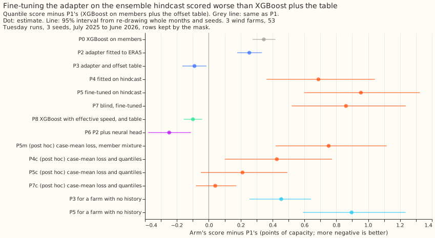
Take-home: a small neural correction of the wind speed, fitted to ERA5 (the weather estimate used for training) and run on the 51 ensemble members, matches XGBoost plus a lookup table of offsets, and fitting the correction on the ensemble hindcast made it worse. The hindcast is 442 daily ensemble forecasts issued from April 2024 to June 2025; the scored year runs from July 2025 to June 2026. Scores are quantile scores (an estimate of the continuous ranked probability score) in points of capacity (1 point is 1% of a farm's capacity); lower is better, and a negative difference means the first arm is better. With the offset table of experiment 259 on top, the adapter fitted to ERA5 (P3) scored 0.09 points better than XGBoost plus the table (P1; 95% interval -0.17 to -0.02). Fine-tuning the adapter on the hindcast (P5) scored 0.95 points worse than P1 (0.60 to 1.32). A repair chosen after seeing the results, which stops the ensemble spread being counted twice, cut that gap to 0.21 points (-0.05 to 0.49), so the adapter is still no better than XGBoost plus the table. Both the mean wind speed and the mean observed power were higher in the scored year than in the hindcast year, which may be why a correction fitted to the hindcast does not carry over; we did not test that.
We asked whether the small neural adapter of experiment
285, which scored better than XGBoost with ERA5 as
the weather, also wins on the production weather input, the ensemble forecast, in the scored year.
The adapter scales and shifts the wind speed that the physics model of a wind farm reads. We fitted
it to ERA5, ran it on every member, mixed the 51 members with equal weights, and added experiment
259's offset table. We also fitted it directly to the ensemble hindcast. The 3 metered wind farms
(W1, W2, W3) are scored on 53 Tuesday runs from July 2025 to June 2026. Verdict partly supported:
the decision rule (P5 beats P1 by at least 0.10) failed, and its fallback (P8 or P5 beats P1 by
under 0.10, with an interval below zero) held for P8.
Arms and rows
- Arms (all on the 51 members, then the spread factor of experiment 33). P0 is XGBoost trained on ERA5 before 2024-04-01, and P1 is P0 plus experiment 259's offset table (both read from experiment 285; this folder's code reproduces them exactly). P2 is the adapter (inputs: wind direction, the 10 m to 100 m speed ratio, 2 m temperature, hour of day) fitted to ERA5; P3 is P2 plus the table. P4 fits the whole physics model and an adapter on the hindcast alone, and P5 fine-tunes P2 on the hindcast; the P4 and P5 adapters also see the lead day and the members' standard deviation of the 100 m speed. P7 is P5 with an adapter that sees the 100 m speed only. P8 is XGBoost with the adapter's effective speed as an extra column, plus the table. P6 is P2 plus experiment 259's neural head (a small neural network that outputs 11 quantile offsets).
- Cross-fit. P4, P5, and P7 take their hindcast predictions from models fitted without the held-out third of the hindcast runs (purged for overlapping valid times), so the spread factor and the residual quantiles never see an in-sample prediction. The scored predictions come from a model fitted to the whole hindcast, stopping on its last 90 days.
- Post hoc arms (added after the results, so not pre-registered). P4m, P5m, and P7m use a loss on the members' mean power. The Sonnet audit found that the fine-tuned arms count the ensemble spread twice: the residual quantiles are fitted to the case-mean forecast (the forecast from the members' mean power) and applied to each member before mixing. That worsened P5's score by 0.39 points at W1 in the auditor's re-run of one seed. P4c, P5c, and P7c repair the double counting by applying the case-mean residual quantiles to the members' mean power and not mixing members.
- Rows. A row is one farm, seed, run, and valid time. The rows are experiment 33's 53 Tuesday
runs, 3 seeds, and 3 farms; "kept" rows (96,479 of 107,121) are those outside experiment 210's
idle-band mask (the half-hours when a farm is idle). Intervals resample whole months of the run
date and the three seeds (50,000 resamples); farms are not resampled. Eight contrasts were
planned, so the Bonferroni level is 99.375%; the 95% intervals the brief asks for are quoted
below, and the planned contrasts' Bonferroni intervals are in
work/score.json. - Weather at lag times. The adapters and XGBoost read the ensemble's own wind, temperature, and hour of day at forecast time; ERA5 is used only to fit models before 2024-04-01, so no lagged past weather is read at forecast time.
Planned contrasts (kept rows, points of capacity, first minus second; negative means the first arm is better)
- C1, P2 minus P0: -0.091 (-0.167 to -0.017). Predicted -0.05 to -0.2. Held.
- C2, P3 minus P1: -0.090 (-0.166 to -0.015). Predicted a gain smaller than 0.1 points. Held: the table takes most of the gain.
- C3, P5 minus P3: +1.044 (0.721 to 1.365). Predicted at most -0.05. Failed in the opposite direction.
- C4, P4 minus P5: -0.266 (-0.361 to -0.188). Predicted positive (P4 worse). Failed: training from scratch scored better than fine-tuning.
- C5, P6 minus P3: -0.159 (-0.283 to -0.041) on the quantile score, +0.005 (-0.037 to 0.043) at the 0.99 pinball loss. Predicted a 0.99 pinball loss at least 10% lower and a score no worse than +0.1. Held on the score (the head helped the middle of the distribution: median error 15.75 against 16.01) and failed at the tail.
- C6, P8 minus P3: -0.010 (-0.034 to 0.014). Predicted at least as good. Held (a tie).
- C7, share of the P3-to-P5 gap that P7 closes: 0.91 (0.77 to 1.06). Predicted under a third. Failed: the blind adapter did as badly as P5, so the extra inputs gave the fine-tuned arm nothing.
- C8, P5 minus P1: +0.954 (0.599 to 1.324). The decision-rule contrast. Failed.
Scores and tail calibration (kept rows unless stated)
- P6 had the lowest score of the pre-registered arms, 11.104, which is 0.248 points better than P1 (95% interval -0.380 to -0.112). It is not the headline, because P6 adds a second neural network (the head), its 5% to 95% coverage is the lowest of any arm (88.5%), and the 0.99 pinball loss did not improve (C5). Experiment 259 found that a table of offsets recovers most of what the head gains.
| Arm | Kept | All rows | Lead 12 to 36 h | q01 pinball | q99 pinball | 5-95% coverage | Below median |
|---|---|---|---|---|---|---|---|
| P1 XGBoost, table | 11.352 | 10.825 | 6.144 | 0.284 | 0.640 | 92.1% | 40.4% |
| P0 XGBoost | 11.697 | 11.061 | 6.292 | 0.284 | 0.681 | 90.8% | 35.1% |
| P2 adapter, ERA5 | 11.606 | 10.988 | 6.323 | 0.287 | 0.683 | 91.3% | 35.1% |
| P3 adapter, table | 11.262 | 10.756 | 6.165 | 0.287 | 0.644 | 92.6% | 40.4% |
| P4 hindcast only | 12.040 | 11.388 | 6.594 | 0.287 | 0.703 | 91.5% | 34.1% |
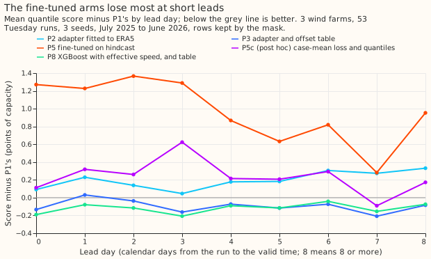
| P5 fine-tuned | 12.306 | 11.559 | 7.267 | 0.289 | 0.726 | 90.8% | 31.8% |
| P7 blind, fine-tuned | 12.213 | 11.513 | 7.516 | 0.290 | 0.702 | 91.4% | 30.1% |
| P8 XGBoost with effective speed, table | 11.253 | 10.746 | 6.062 | 0.283 | 0.639 | 92.0% | 40.7% |
| P6 P2 plus neural head | 11.104 | 10.801 | 5.891 | 0.284 | 0.649 | 88.5% | 46.9% |
| P5m post hoc, mixture | 12.104 | 11.351 | 6.536 | 0.287 | 0.691 | 91.8% | 28.6% |
| P4c post hoc | 11.779 | 11.199 | 6.350 | 0.287 | 0.690 | 90.9% | 38.9% |
| P5c post hoc | 11.564 | 11.009 | 6.435 | 0.287 | 0.692 | 91.2% | 38.8% |
| P7c post hoc | 11.393 | 10.916 | 6.498 | 0.287 | 0.669 | 91.6% | 40.4% |
- P5c against the other arms (post hoc). P5c minus P3 is +0.301 (0.071 to 0.539), P5c minus P1 is +0.212 (-0.049 to 0.493), and P5c minus P2 is -0.043 (-0.282 to 0.219): once the double counting is repaired, fine-tuning on the hindcast adds nothing over the ERA5 adapter, and the blind P7c scores 0.171 better than P5c (0.007 to 0.342), so the adapter's extra inputs add nothing.
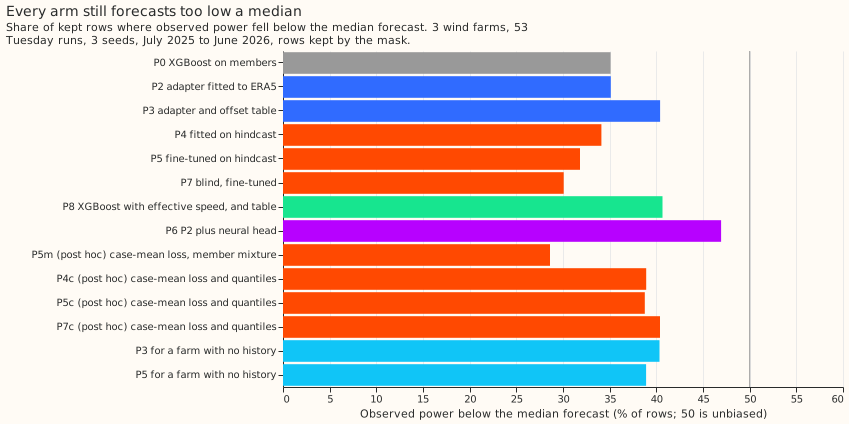
- The tails. Every arm's 0.99 pinball loss is between 0.639 and 0.726, and the best arms (P1, P3, P8) are within 0.01 of each other. Every arm's median forecast is too low: observed power was below the median forecast on 28.6% to 46.9% of rows (50% is unbiased), and P6 is the closest at 46.9% with the lowest 5% to 95% coverage (88.5%).
- A farm with no history: P3 scored 0.544 points worse when fitted to the other two farms. Fitted to the other two farms with no idle layer, P3 scored 11.807 (+0.544, 0.373 to 0.721 against P3). P5 scored 12.248 (+0.441, 0.232 to 0.686 against the P3 version). The no-history version is a pooled pipeline, so each contrast mixes pooling, no idle layer, and a fixed spread factor. Only the turbine count and rating from the Renewable Energy Planning Database would be known for such a farm; the adapter above was not given them.
- Curtailment cost. Not scored: no arm's output was run through
studies.node_curtailmentbecause the metric scores a node with its generators and not three farms alone.
Checks and the audit
- Median minus mean forecast (kept rows, pooled over the farms, points of capacity): P0 -4.97, P1 -4.81, P2 -4.82, P3 -4.71, P5c -4.61, P6 -3.91, P8 -4.72. The offset table moves the median by about 0.1 to 0.2 points, as experiment 259 found.
- Mean-forecast error beside each quantile contrast (C2, C3, C5, C6). The mean-forecast absolute error moves the same way as the score in C2 (-0.116), C3 (+0.888), and C6 (-0.006), and in the opposite direction in C5 (+0.133 against a score change of -0.159), because the head lowers the median's error (-0.258) and not the mean's.
- Audit triggers fired: the blind control P7 scored no worse than P5, C3 and C4 contradicted the
prediction, and P4 beat P5, which starts from more. A fresh Sonnet agent audited the code and the
results; the maintainer asked for Sonnet only, so no Opus audit ran. Its findings and their
triage:
- The member mixture counts the ensemble spread twice for P4, P5, and P7. Accepted. The auditor's re-run of one P5 seed at W1 scored 11.72 with the mixture and 11.33 with the case-mean quantiles (not stored). The stored W1 scores are 11.707 for P5, 11.305 for P5m, and 10.833 for P5c. The repaired arms P4c, P5c, and P7c are post hoc, and the table above shows they do not change the conclusion.
- The hindcast year differs from the scored year. Accepted. The shift table below
(
work/shift.json, frome00303_shift.py) shows that the mean observed fraction of capacity and the ensemble-mean speed both rose. - No mismatch between the hindcast and scored adapter inputs, and early stopping on one spring season is not the cause. No change.
- P5 has two extra inputs that P2 lacks (lead day and spread), so C3 mixes the inputs with fine-tuning. Accepted as a caveat. P7, which has none of them, scored the same as P5 (C7).
- P6's base was chosen from P2, P4, and P5 on their hindcast scores (P3 is P2 plus the table the head replaces). Accepted as designed. The hindcast scores of P4 and P5 are slightly in sample for the residual quantiles, and P2 won regardless.
| Farm | Mean ensemble 100 m speed, hindcast then scored year (m/s) | Mean observed fraction of capacity, hindcast then scored year |
|---|---|---|
| W1 | 6.73 then 7.02 | 0.198 then 0.254 |
| W2 | 7.42 then 7.70 | 0.246 then 0.284 |
| W3 | 7.74 then 8.09 | 0.214 then 0.251 |
What to try next
- Fit the correction to many years of ERA5 and to the ensemble hindcast together, with an indicator saying whether each row is ERA5 or ensemble data, so the correction does not depend on one year's relation between speed and power.
- Find the reason the scored year had higher mean speed and mean power (turbine availability, a change of ensemble model cycle, or ERA5 drift) before trusting a one-year fit.
- Give XGBoost the effective speed (P8) if the small gain of 0.099 points is wanted. It needs no second training stage, and the threshold for porting a change that adds a neural network is 0.10 points, so the gain falls just below it.