Gap robustness of the convex model with a Kalman filter: coast or fall back
Take-home: when power readings stop, keep the Kalman filter running without new readings
("coasting") and widen the bands. At each of the four gap lengths tested (3, 6, 24, and 72 hours)
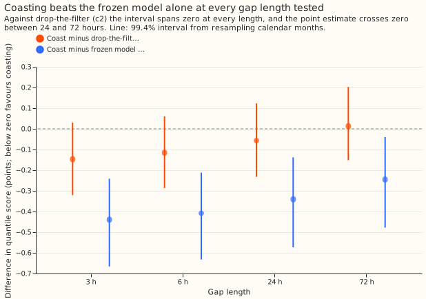
that forecast scored 0.25 to 0.44 points of quantile score better than the convex demand model with
no correction. A quantile score is an error measure in percent of the substation's effective
capacity, and lower is better. Whether dropping only the filter would beat coasting at about 72
hours could not be told. The formal verdict is inconclusive: each comparison planned in advance
against the same forecast with the filter dropped has an interval that includes zero.
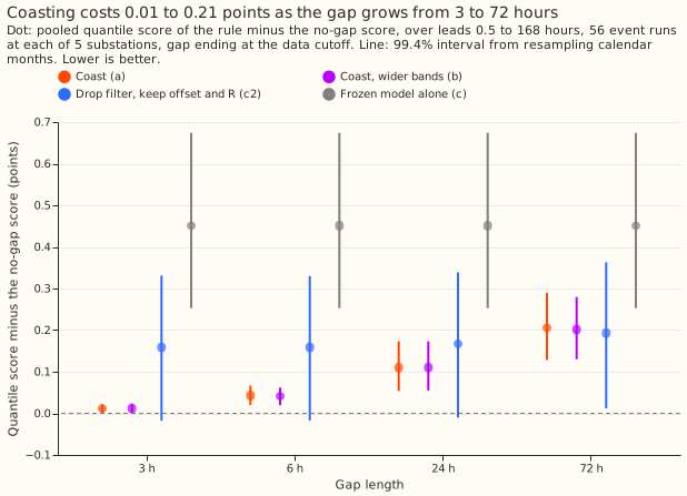
We asked what a live forecast should do when power readings go missing: let the filter coast, coast and also widen the bands, or drop the filter. The demand model is the convex generalised additive model of experiment 111 with a Kalman filter on its recent errors (GAM-K, a method re-implemented from de Vilmarest and Wintenberger (2022)), plus the winter night offset and recipe R of arm D of experiment 155. We hid every reading in the 3, 6, 24, or 72 hours ending at the forecast's data cutoff (the time of the last usable reading), for up to 56 forecast runs (events) at each of five substations (275 events in all), and scored the forecast over the next 168 hours. With coasting, the quantile score (2.747 points with no gap) worsened by 0.011 points after a 3-hour gap and by 0.206 points after a 72-hour gap. With the filter dropped, it worsened by 0.158 to 0.193 points at every gap length.
Headline numbers
All differences are in points of quantile score, over leads of 0.5 to 168 hours. An interval is the 99.4% bootstrap interval, resampled by calendar month, and "spans zero" means it includes zero. Rule letters: (a) coast, (b) coast with wider bands, (c2) drop the filter, (c) the frozen model alone.
- Rules. (a) The filter on the gapped readings, then the winter night offset (a monthly refitted correction to winter night forecasts) and recipe R (subtract 0.75 times the mean forecast-error profile of the previous 14 days). (b) Rule (a) with the quantile offsets widened by the filter's variance growth since the last reading. (c2) Rule (a) with the filter dropped. (c) The convex demand model with no filter, offset, or recipe R, called the frozen model. The plan below fixes these rules before any score was read.
- Events. Five decision substations (D5, D10, D11, D14, and D16) with 53 to 56 events each (275 in all), one randomly drawn forecast run per 8-day block. The gap ends at the data cutoff (k = 0, where k is the number of hours between the gap's end and the cutoff). The spread tables, which hold the quantile offsets from the mean, come from the no-gap forecast of experiment 136's arm A2.
- Absolute scores. No gap 2.747. Rule (a) 2.758, 2.790, 2.857, and 2.953 at 3, 6, 24, and 72 hours. Rule (b) 2.759, 2.788, 2.857, and 2.948. Rule (c2) 2.905, 2.905, 2.914, and 2.940. Rule (c) 3.198, whatever the gap.
- Coasting minus dropping the filter (rule (a) minus rule (c2)). 3 hours -0.147 (-0.321 to +0.030). 6 hours -0.116 (-0.287 to +0.060). 24 hours -0.057 (-0.232 to +0.123). 72 hours +0.013 (-0.152 to +0.203). All four span zero, so no crossover length is established and the pre-registered test fails. Over leads under 24 hours the contrast is below zero at 3, 6, and 24 hours (-0.480, -0.401, and -0.295) and spans zero at 72 hours (-0.167, -0.353 to +0.022).
- Coasting minus the frozen model alone (rule (a) minus rule (c)). -0.439 (-0.666 to -0.241), -0.408, -0.341, and -0.245 (-0.478 to -0.040) at 3, 6, 24, and 72 hours. The plan treats this contrast as descriptive.
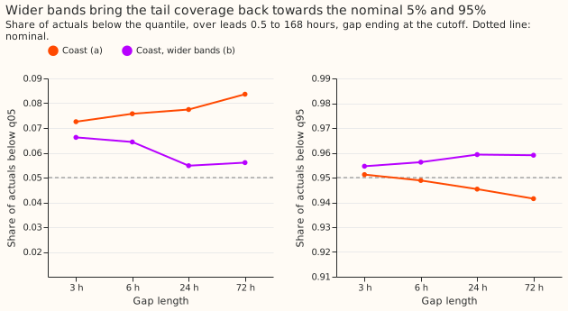
- Wider bands (rule (b) minus rule (a)). The score changes by -0.004 to +0.000 at every length, and every interval spans zero (72 hours: -0.004, -0.033 to +0.014). The share of actual readings below the predicted 5% quantile (q05) changes by -0.006, -0.011, -0.023, and -0.028 (24 hours: -0.032 to -0.015), and the share below q95 by +0.003, +0.007, +0.014, and +0.018.
- Coverage. Under rule (a), 7.3%, 7.6%, 7.7%, and 8.4% of actual readings fall below q05 at the four gap lengths, and 95.1%, 94.9%, 94.5%, and 94.2% fall below q95. Under rule (b) the shares are 6.6%, 6.4%, 5.5%, and 5.6% below q05 and 95.5%, 95.6%, 95.9%, and 95.9% below q95. With no gap the shares are 7.1% and 95.1%.
- Rule (b) meets the plan's criterion for replacing rule (a). The mean absolute distance of the q05 and q95 shares from nominal is 0.016 for rule (a) and 0.007 for rule (b) at 24 hours, and 0.021 and 0.008 at 72 hours. The intervals of the coverage differences exclude zero (24 hours: q05 -0.032 to -0.015, q95 +0.010 to +0.018), and the score difference is at most +0.000 against the +0.01 limit. The coverage differences use the month-resampled interval rather than the plan's binomial standard error, because forecast errors in the same month are correlated.
- Tails under rule (a), 3 to 72 hours. The pinball loss at the 1% quantile is 0.222 to 0.257 and at the 99% quantile 0.231 to 0.242. The share of readings below the 1% quantile is 2.5% to 3.2% and below the 99% quantile 98.1% to 98.4%. Under rule (b) those shares are 1.6% to 2.2% and 98.6% to 98.8%.
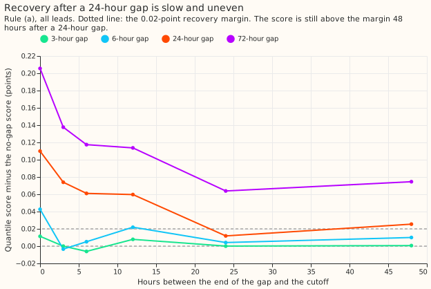
- Recovery. Recovery is the smallest k from which the score stays within 0.02 points of the no-gap score. After a 24-hour gap, rule (a) minus the no-gap score is +0.110, +0.074, +0.061, +0.060, +0.012, and +0.025 points when k is 0, 3, 6, 12, 24, and 48 hours, so the pre-registered recovery (6 hours or less) fails. The filter alone (rule (a0)) is within 0.02 points from 24 hours on. After a 3-hour gap, recovery takes 0 hours; after a 6-hour gap, 24 hours; after a 72-hour gap, the score has not recovered at 48 hours.
- Differences between substations (rule (a) minus rule (c2)). At 3 hours: D10 -0.171, D11 -0.228, D14 -0.342, D16 +0.056, and D5 -0.040. At 72 hours: D10 +0.033, D11 -0.012, D14 -0.235, D16 +0.222, and D5 +0.061.
Checks
- Median minus mean forecast. Exactly 0.000 at every substation and rule, because the centred spread table places the median at the mean. The check cannot expose a shifted forecast here.
- Mean-error contrast beside the quantile score. Rule (a) minus rule (c2) on the absolute error of the mean forecast is -0.270 (below zero), -0.219, -0.124, and -0.006 points at 3, 6, 24, and 72 hours. The sign matches the quantile-score contrast at 3, 6, and 24 hours and differs at 72 hours, where both contrasts span zero (mean error -0.233 to +0.234).
- Controls. The rebuilt no-gap forecast reproduces experiment 155's stored arm D exactly (the largest mean difference is 0.0 at all five substations). Widening by zero variance leaves the quantiles unchanged. Replacing every actual at or after a run's origin with random numbers leaves the mean forecasts of three tested runs unchanged.
- Audit. The skill's audit check fired because leaving out D14 moves the 24-hour contrast from -0.057 to +0.001, and leaving out D16 moves the 72-hour contrast from +0.013 to -0.040. An independent reviewer re-derived the contrasts from the stored forecasts, and they match to 4 decimal places. The reviewer found no path by which future readings reach the forecast. The reviewer traced both sign changes and the 72-hour sign to one date, 2026-01-13, at D5 and D16 (the first finding below). Both contrasts span zero, so the verdict does not change.
Audit findings
- One switching date carries the 72-hour sign and both leave-one-out flips. On 2026-01-13 the
no-gap forecast scored 15.3 points at D16 and 16.9 at D5, against 1.7 and 7.6 for rule (c2). The
14 days before that cutoff all fall inside a hand-filtered switching event, but the filter still
read those readings. It had learned the changed load, moving its level estimate by +22 points at
D16 and by -9 points at D5. The hidden gap did not cause the large errors. Dropping that date
after the fact (a post-hoc cut, not the verdict) gives rule (a) minus rule (c2) of -0.204
(-0.363 to -0.059) at 3 hours and -0.171 (-0.327 to -0.023) at 6 hours, both below zero. The
same cut gives -0.112 and -0.037 at 24 and 72 hours, both spanning zero. On that cut the
pre-registered rule would read
partly supported. The 72-hour sign, coasting worse, is not a basis for a rule that drops the filter. - At 3 and 6 hours the contrasts mostly measure the filter's no-gap value. Every forecast starts at 09:00 UTC and its data cutoff is 05:30 UTC, so a 3-hour gap covers only the night hour band (and the morning band in summer time). A band here is a block of hours of the day that gets its own correction. The contrast splits into +0.011 from the gap and -0.158 from the filter's no-gap advantage. A gap ending in the evening would test more.
- The widening is crude. Most of the extra variance comes from the filter's short-lived transient component. The method applies it unchanged at every lead up to 168 hours, although it should shrink as the lead grows. Part of the coverage gain also corrects under-coverage that the no-gap forecast already has (7.1% of readings fall below q05, against a target of 5%).
Caveats
- Gaps are injected, not real. Hiding readings in clean data does not reproduce a stuck meter, a communications fault that backfills later, or a gap at a switching event.
- The demand model's monthly refits continue during a gap. A gap that spans a refit cut would also thin the training data, and that effect is not modelled.
- The quantile offsets differ slightly from those of the no-gap forecast. The offsets differ by up to 1.4 points, because the winter night offset and recipe R move on rows near a gap. Rule (c) has its own table.
- Hidden readings stay hidden for later runs. A telemetry backfill would restore them, so the recovery shown is a worst case.
- The 275 events lie in 18 calendar months, and the intervals resample those months.
What to try next
- Real outages would be a more realistic test. They could be scored once the cleaned power table's outage periods are listed. Resolving the 72-hour question would take more events or real gaps.
- Masking switching readings from the filter could be tested. One date shows that unmasked readings can raise the quantile score by 14 points. A test that masks them would also settle the 72-hour comparison.
- A small neural network could shorten the recovery. It would take the filter state and the hours since the last reading and rescale how fast the transient decays. If it works, the score after a 24-hour gap would be within 0.02 points of the no-gap score 12 hours after the gap ends.
Planned design
The design below was fixed before any score was read. Two details changed after the plan review and before any run: the comparator for the headline contrasts is rule (c2), and the gap hides the actuals from the offset and recipe R as well as the filter.
Question. In production the convex demand model with a Kalman filter (GAM-K, the Kalman filter on recent errors of experiment 111; the method re-implements de Vilmarest and Wintenberger (2022)) will sometimes receive no power readings for hours or days. We ask which rule to serve then, and whether a gap length exists beyond which the filter should be dropped.
Design.
- Inputs. The unfiltered forecast of every run (experiment 136's A2: the T-all fits driven by the calibrated ensemble mean), rebuilt from the stored fits and ensemble arrays as in experiment 197, and the filter's residual stream. The full pipeline is the arm D of experiment 155: the filter, the winter night offset, and recipe R (minus 0.75 times the 14-day mean error profile).
- Events. For each substation the origins of the replicate and scored runs (excluding the every-fifth-day stride runs and any origin before 2024-07-16) are cut into blocks of 8 days, and one run is drawn at random (seed 205) from the first 3 days of each block, so two events are at least 6 days apart and no gap window reaches the previous event's cutoff. The same event runs are used for every gap length and rule.
- Gap. The readings of all four hour bands are removed for the L hours up to k hours before the event run's data cutoff, with L in {3, 6, 24, 72} and k in {0, 3, 6, 12, 24, 48}; all 24 combinations are scored, and the headline contrasts use k = 0. One filter pass per (substation, L, k) applies the gaps of all that substation's events together, which is equivalent to one pass per event because the windows do not overlap.
- What each stage sees. The filter reads the gapped stream. The winter night offset is refitted monthly on the errors of the earlier rows of the gapped timeline, as in experiment 155, with the actuals inside gaps hidden. Rows of the tuning months keep the no-gap filter's forecast, so every rule's spread table is the no-gap one even where a gap reaches back into a tuning month. Recipe R is recomputed from the gapped timeline: it uses the errors of the earlier runs from the gapped filter, and the actuals whose valid time falls inside any gap are hidden from its error blocks (a block with fewer than 40 readings is unusable, as in experiment 155). Scoring reads the true actuals of the event run's own rows, which all fall after its origin.
- Rules. Each rule's offset, R profile, and spread come from that rule's own forecast errors. (a) Coast: the gapped filter, then the offset and R. (b) Coast with widened bands: rule (a)'s 11 quantiles with their offsets from the mean multiplied by sqrt(1 + v / s^2), where s = (q95 - q05) / 3.29 of the row, in points, and v is the extra predictive variance of the level and transient, in points squared, over the no-gap filter at the same cutoff. With n and n0 the half-hours from the target band's last reading to the cutoff in the gapped and the no-gap stream, v = max(0, w(n) - w(n0)), where w(n) = q n / 48 + sigma_z^2 (1 - phi^(2n)) / (1 - phi^2), using the single pooled setting (q, phi, sigma_z) of experiment 133 that arm A uses. (c2) The no-gap pipeline with the filter dropped for all runs: the frozen GAM plus its own offset and R. (c) The frozen GAM alone, with a spread refitted on its tuning months, no offset and no R. Secondary: (a0) and (b0) are (a) and (b) with the filter alone, no offset and no R, spread refitted on the filtered tuning errors.
- Scored. Five decision substations, D5, D10, D11, D14, and D16, over leads 0.5 to 168 hours, then under 24 hours and 12 to 36 hours; per-substation contrasts and the number of events per substation and length are reported beside the pooled ones.
- Compute. CPU only, 4 cores, no new fit; the filter re-runs on a masked stream per (substation, L, k).
Prior advice followed: the Kalman state is the one of experiment 111 with the POOL setting (experiment 136, A2); no faster level is used (experiment 197); recipe R at every lead and no offset on top of R is experiment 155's finding, but this plan keeps arm D, the pipeline that experiment 155 tested, so the offset stays in the gapped pipeline and the comparison stays with the stored arm D.