Experiment 135: does fitting the demand model through the Kalman filter beat fitting it first and filtering after?
Fitting the demand model so that it is judged after the Kalman filter's correction made the
day-ahead forecast much worse, and tying it to the ordinary fit removed the damage and added no
gain.
The quantile score at leads 12 to 36 hours (our error score for a forecast with uncertainty bands,
in points of capacity; smaller is better) rose by 5.4 points without the tie (arm J1; 97.5% interval
+3.3 to +8.5). With a ridge penalty that ties the fit to the two-stage coefficients (arm J2), the
score changed by -0.0045 points (-0.013 to +0.003), which cannot be told from zero. The verdict is
not supported. The two-stage design stays: fit the demand model, then filter its residuals.
We asked whether the convex demand model forecasts the next day better when its coefficients are chosen to minimise the error that remains after the Kalman filter has corrected the forecast. The demand model is GAM-K, the convex additive model with a Kalman filter on its residuals from experiment 111. The filter tracks a slowly moving level and a quickly decaying transient of the demand model's error in each of the 4 hour bands of the day, with the noise settings that experiment 133 chose. In the two-stage design, the demand model is fitted first and the filter then runs on its residuals. For fixed noise settings the filter is linear in the residuals, so the joint fit is an exact bounded quadratic problem. We solved it on a graphics processing unit (GPU) with no gradient descent. The idea follows de Vilmarest and Goude (2022), who run a state-space correction on the residuals of a generalised additive model for electricity load. They correct the residuals after fitting, and this experiment fits through the correction.
The experiment compared three arms on fold_a_daily_gap_v1 at the five decision substations (D5,
D10, D11, D14, and D16, with D9 beside them):
- TS: the two-stage fit, as in experiment 111, with experiment 133's filter settings (its GRID arm, which chose the settings per substation by next-day score).
- J1: the joint fit with no tie to TS.
- J2: the joint fit plus a penalty (a ridge) that pulls the coefficients towards TS's coefficients, with a weight chosen per substation from {0.1, 0.3, 1, 3} by the score on the tuning months (odd months of 2024-07 to 2025-06). The choice was 3 at five substations (D5, D9, D10, D11, and D14) and 0.3 at D16.
Results
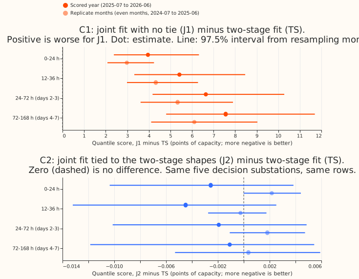
- J1 scores worse at every lead and at every substation. C1 (J1 minus TS) at 12 to 36 hours is +5.419 points (97.5% interval +3.330 to +8.465) in the scored year (2025-07 to 2026-06), and none of the five substations improve. In the replicate months (even months of 2024-07 to 2025-06) it is +4.323 (+2.988 to +6.281). The gap grows with lead, from +3.96 at 0 to 24 hours to +7.56 at days 4 to 7 (figure 1). The absolute quantile score at 12 to 36 hours is 7.907 for J1 against 2.488 for TS. Over all leads (0.5 to 168 hours), J1 scores 9.563 and TS scores 2.783. D9, scored beside the decision substations, shows the same pattern (J1 6.009 against 2.151 at 12 to 36 hours).
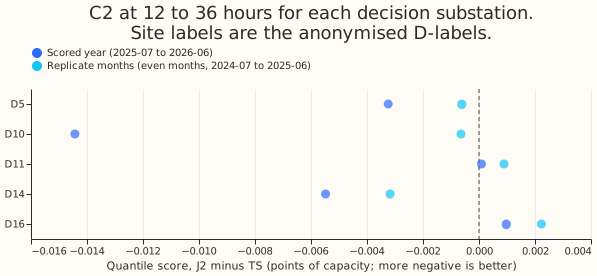
- J2 is indistinguishable from TS. C2 (J2 minus TS) at 12 to 36 hours is -0.0045 points (-0.0132 to +0.0025) in the scored year, with three of five substations improving, and -0.0002 (-0.0027 to +0.0018) in the replicate months, with three of five. The interval rules out a worsening of the score by more than 0.003 points and an improvement by more than 0.013 points. Over all leads, C2 is -0.0015 (-0.0106 to +0.0048), within the non-inferiority bound of +0.02. D10 contributes most of the scored-year difference (-0.0144, figure 2), and leaving D10 out leaves a mean of about -0.002.
- The tuning months prefer the strongest tie on the grid. The mean tuning-month score is 2.7136 for ridge weight 0.1, 2.7067 for 0.3, 2.7028 for 1, and 2.7020 for 3, against 2.7028 for TS (J1 is 8.200). The score falls as the tie tightens and reaches TS's, so the tuning months prefer the two-stage fit. The best weight lies at the edge of the grid at five of six substations.
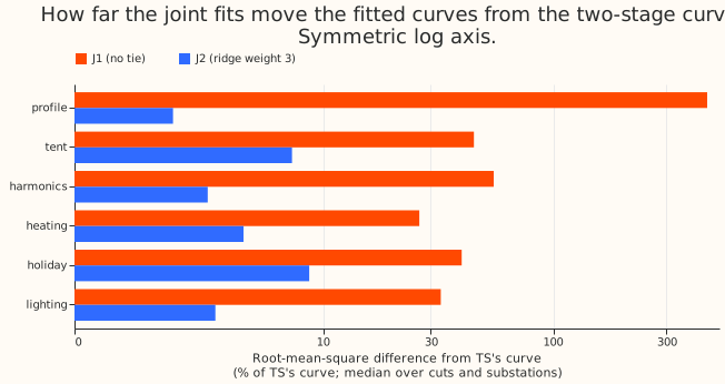
- J1's fitted curves move far from the two-stage curves, and J2's barely move. For each term, we took the root-mean-square difference between a joint fit's curve and TS's curve, as a share of the spread of TS's curve, and then the median over the 27 monthly refits and five substations. For J1 the shares are 444% for the weekly profile, 46% for the tent (a term for the temperature response), 56% for the harmonics (the yearly cycle), 27% for heating, 41% for the holiday term, and 33% for lighting. For J2 at weight 3 they are 2%, 7%, 3%, 4%, 9%, and 3% (figure 3). Most of J1's weekly-profile difference is a constant offset: a median of 51 points of capacity as it stands, against 10 points once the offset is removed. The filter's level absorbs that offset.
- Breakouts, at 12 to 36 hours in the scored year (descriptive). C1 and C2 are:
- Winter (November to March): +6.53 (+2.17 to +12.93) and -0.007 (-0.023 to +0.004).
- Winter nights: +1.85 (+0.05 to +4.26) and -0.004 (-0.025 to +0.007).
- Cold nights: +2.44 (+0.64 to +5.80) and -0.017 (-0.048 to +0.013).
- Christmas and bank holidays: +4.32 (+3.88 to +5.15) and -0.061 (-0.209 to +0.023).
- Tails. J2's coverage matches TS's to within 0.001 at every quantile shown, so the cold-night
shortfall of the 0.95 quantile that experiment
125
and experiment 133 found is unchanged. The values for TS, J1, and J2 are:
- 0.95 quantile: 0.942, 0.886, and 0.941 over all hours, and 0.864, 0.945, and 0.864 on cold nights.
- 0.01 quantile: 0.020, 0.046, and 0.020.
- 0.05 quantile: 0.064, 0.078, and 0.064.
Checks
- P1, reproduction (blocking): passed. TS's scored-year mean forecasts equal experiment 111's stored GAM-K rows, and its mean and median forecasts equal experiment 133's GRID rows, with a maximum absolute difference of 0 at all five decision substations.
- P2, the linear filter equals the filter: passed. Unit tests in
packages/studies/tests/test_dp_joint_fit.pymatch the corrected loss torun_kalmanandcorrection_atto a relative 1e-9 in float64, with gaps in the readings and a binding variance floor. They also matchfit_gamto 1e-6 when the filter is switched off. - P3, the solved loss is the true loss: passed. At all five substations, the loss of the filter run on the joint solution's residuals (the summed squared error after correction) is lower than the loss at a perturbed set of coefficients and lower than the loss at TS's coefficients. At D10 the three values are 1,120,985, 1,121,407, and 1,150,502. The fit does minimise the loss it was given, so J1's poor score comes from that loss and not from the solver.
- P4, known answer: failed for J1, passed for J2. The target was simulated from TS's own curves plus a slow level, a decaying day anomaly, and white noise. The summed centred root-mean-square error of the recovered curves over the five substations was 36.6 points of capacity for J1, 11.2 for TS, and 10.4 for J2. J1 loses even when the assumptions of the joint design hold. The weekly profile accounts for 27.3 of J1's 36.6.
- Absorption control: J1 failed in 4 of 15 substation-cut pairs, and J2 in none. A term fails the control only if it moves by more than twice its noise floor, which is how far it moves when the training cut-off moves back by 7 days. J1's noise floors are large, so J1 can move a long way without failing. J1's weekly-profile noise floor has a median of 19 points of capacity and a maximum of 95, against 1 point for J2 and TS. The J1 failures are D10 at the 2025-01, 2025-07, and 2026-01 cuts and D5 at the 2026-01 cut. A term had a noise floor above 1 point (unidentified) in 14 of 15 pairs for J1 and 10 of 15 for J2. The holiday term has a noise floor above 1 point in 11 of 15 pairs for J1 and 10 of 15 for J2 and TS, because few holidays fall in a training window.
- Predictions against results. C1 was predicted at -0.05 to +0.02 points, and the result of +5.4 is more than 100 times the top of that range. C2 was predicted at -0.03 to +0.01 and came out at -0.0045, inside the range. J1's curves were predicted to differ from TS's by 5% to 15% of each term's spread, and they differ by 27% to 444%. J2's were predicted to differ by under 5%, and that held for four terms but failed for the tent (7%) and the holiday term (9%). The absorption prediction (J1 fails, J2 does not) held.
- Error of the mean forecast beside each contrast (12 to 36 hours, scored year). The mean absolute error is 4.374 for TS, 11.027 for J1, and 4.367 for J2, in points of capacity. The C2 contrast on the mean forecast's error is -0.0073 (-0.0207 to +0.0032), the same sign as the quantile-score contrast, so the audit trigger for a disagreement did not fire. The median forecast minus the mean forecast is -0.156 for TS at D5 and -0.154 for J2, against -0.319 for J1, and is within 0.05 for TS and J2 at the other four substations.
- Audit triggers. Trigger 1 (a control fails) fired, because P4 failed for J1. Trigger 2 (a result against its own prediction) fired for C1. The shape distance, the noise floors, and P4 support the explanation that the filter absorbs a shift of the slow terms, so the loss leaves them to the penalty alone. No variant of the loss was run to test that explanation. Trigger 4 (one substation drives the contrast) did not change a verdict: C1 is positive at every substation, and C2's full interval spans zero while the mean of the four substations other than D10 is -0.0019 (an interval for those four was not computed). No Opus audit was run, by agreement with the experiment manager, so triggers 1 and 2 are unresolved caveats.
- Biases stated in advance. At the joint fit, the filter reads in-sample residuals from the training weather (the fifth-generation European Centre reanalysis, ERA5, and the Copernicus Atmosphere Monitoring Service, CAMS). At forecast time it reads out-of-sample residuals from the analysis proxy, the stand-in for past weather. The noise settings were chosen on TS's own residual stream, which favours TS. J2 is a family of fits, with the tie weight chosen on the tuning months. These biases favour TS, or tie J2 to TS, so they cannot explain J1's poor score. They do limit what a null for J2 says about a joint fit with retuned noise settings.
- Retraining schedule and cost. All arms refit the convex model monthly, as in experiment 111. The joint fits of all five weights (J1 and four J2) took 0.33 GPU hours in total, about 3.3 minutes per substation for 27 refits. The fits, tuning, forecasts, scoring, and controls together took about an hour and a half of wall-clock time.
What the next experiment should answer
- Whether learning the filter's noise settings together with the coefficients helps. This experiment held the settings fixed at experiment 133's values, so a null for J2 does not rule out that joint learning helps. That experiment would need a loss in which the slow terms stay identified, and J1's failure suggests tying them to a reference fit.
- Whether a ridge weight above 3 changes J2. The tuning months preferred the strongest tie at five of six substations, so a wider grid would show whether a tie stronger than weight 3 gives any improvement.