Experiment 85: do cheaper retraining schedules rank arms the way weekly retraining does? (SPD1)

Refitting the XGBoost demand-forecasting model monthly on the latest 12 months of data (150 boosting rounds), or weekly on the whole history with 150 rounds at a higher learning rate, gives a gap between monthly and weekly retraining within 0.01 points of the gap that full weekly retraining gives, at 0.03 to 0.31 of its fit time. Refitting only quarterly scores much worse. The effect of starting the XGBoost model from zero, not from XGBoost's estimated value, is too small on these rows to rank any schedule, so the agreement on that contrast says nothing.

We asked whether research experiments can use a cheaper retraining schedule instead of weekly retraining. For the 16 Primary substations (which step 33 kV down to 11 kV) we refitted the XGBoost demand model (N1: one XGBoost model per substation, trained on the ECMWF ensemble control forecast) under six cheaper schedules. We then compared the gaps in the quantile score between arms under each schedule with the gaps stored weekly retraining gives, on 158 daily forecast runs from July 2025 to June 2026. The quantile score estimates the continuous ranked probability score from nine quantile levels, in percentage points of the substation's capacity (lower is better). The verdict is partly supported. By the rule fixed in advance every schedule passes. The pass on the starting-value contrast is empty, so only the cadence contrast supports the claim. The experiment leaves out the am-against-d0 contrast of experiment 64 (a demand model given a solar forecast, against the best guess) and the five-model blend of experiment 49, because experiment 64 has no weekly reference and the blend mixes schedules.

Results

• Terms: the cadence gap is the monthly arm's score minus the weekly arm's. The starting-value gap is the score of a model whose boosting starts from zero minus that of a model that starts from XGBoost's estimate from the training labels. A 12-month window means each refit trains on the latest 12 months only (150 rounds, learning rate 0.15). The full setting trains on the whole history (500 rounds, learning rate 0.05).
• Rows: 16 Primary substations, 158 runs, N1 model with the spread factor 1.15 (a fixed widening of the quantiles) and no 14-day correction. Every weekly arm refits at the 28 weekly dates that experiment 80's stored zero-start arm holds, and every contrast keeps the runs those refits serve.
• Noise floor: 0.01 points, the minimum the plan sets. The measured differences between repeats are 0.0004 to 0.0013. A repeat of the 12-month-window monthly fit scored 5.563 against 5.563, and its zero-start repeat 5.547 against 5.546. The tolerance is 0.05.
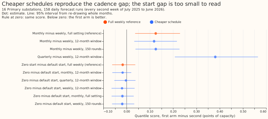
• Cadence gap: the full-setting reference is +0.125 (95% interval +0.036 to +0.229). The 12-month window gives +0.118 and the 150-round whole-history recipe +0.125, so both agree with the reference. Quarterly minus weekly refits on the 12-month window, descriptive because no full-quarterly reference exists, is +0.381 (+0.207 to +0.565).
• Starting-value gap: the reference is -0.017 (-0.062 to +0.037), smaller than the -0.07 the plan predicted. Every schedule gives between -0.003 and -0.020, so each agrees under the rule for an unresolved reference (an estimate within 0.05 of zero). Any estimate within 0.05 of zero passes, so the agreement is weak evidence.
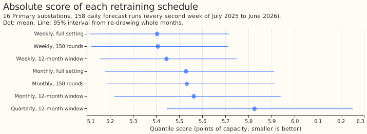
• Pass table: monthly 12-month window 2 of 2 contrasts, weekly 150 rounds 2 of 2, weekly 12-month window 1 of 1, quarterly 1 of 1, full monthly 1 of 1 (the last three on starting value only). The plan also predicted that quarterly refits would score 0.10 to 0.20 above monthly and that the monthly gap would lie within 0.05 of the reference. Quarterly scored 0.263 above monthly, and the monthly gap was within 0.01 of the reference.

Arm	Score	95% interval	Coverage of q05 to q95	Pinball at q05	Pinball at q95
Weekly, full setting	5.405	5.111 to 5.716	0.889	0.910	1.236
Weekly, 150 rounds	5.408	5.119 to 5.711	0.897	0.908	1.233
Weekly, 12-month window	5.445	5.157 to 5.749	0.889	0.912	1.245
Monthly, full setting	5.530	5.179 to 5.912	0.888	0.907	1.294
Monthly, 150 rounds	5.533	5.185 to 5.913	0.896	0.911	1.288
Monthly, 12-month window	5.563	5.219 to 5.939	0.889	0.920	1.288
Quarterly, 12-month window	5.826	5.446 to 6.252	0.883	0.946	1.372

Cost

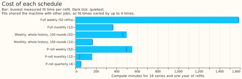
• Fit time of one refit (one series, 2 threads): 114 s at the full setting, 33 to 36 s for the 150-round whole-history recipe, and 13 to 51 s for the 12-month window. Other jobs shared the machine, so the same recipe varied by up to 4 times.
• A year for 16 series: full weekly about 1,590 compute minutes (the full monthly fit time times 52, not measured separately), full monthly 366, weekly 150 rounds 460 to 500, monthly 12-month window 42 to 164, quarterly 54.
• Against the one-third rule: monthly 12-month window (0.03 to 0.10 of full weekly's fit time) and weekly 150 rounds (0.29 to 0.31) pass. Weekly on the 12-month window (0.31 to 0.35) is borderline.

Caveats

• Departure from the written rule: by the pre-registered rule every schedule passes, and quarterly (0.034 of full weekly's cost) would become the default for the starting-value contrast. We do not adopt that default. The rule is vacuous for a gap of 0.017. The descriptive quarterly gap of 0.38 is also large.
• Starting value is untested: the stored weekly zero-start arm covers half of the weeks, and the gap on those runs is within the noise. A later experiment should test schedules on a contrast of 0.1 points or more that has a stored weekly reference.
• One series class, one seed: the experiment covers the cadence and starting-value contrasts for Primary N1 demand only. Tail scores stop at q05 and q95, because the stored quantile models have nine levels from 0.05 to 0.95.
• Cost is noisy: the plan priced a schedule by the mean fit time of its recipe. Identical recipes ran up to 4 times apart because other jobs shared the machine, so we give a range, and each cost is accurate only to within a factor of about 4.

Recommended R&D defaults

• Feature and recipe contrasts of 0.05 points or more: use monthly refits on a 12-month window with 150 rounds and learning rate 0.15. The schedule reproduced the cadence gap to within 0.01 and repeated to within 0.001. A weekly year costs about 1,590 compute minutes and this schedule saves 1,420 to 1,545 of them (90 to 97%). Only the cadence contrast was tested, so a feature contrast is assumed to carry over.
• Contrasts about cadence, retraining rules, or how fast an XGBoost model adapts: use the weekly refit on the whole history with 150 rounds and learning rate 0.15. The schedule scored within 0.003 of full weekly and saves about 1,090 minutes (69%). Experiment 34 found that the gain from adding weekly-analogue inputs (0.05 on a frozen model) shrank to 0.01 under monthly retraining, so a conclusion about recent-data features, the 14-day correction, the training window, or the half-life can change with the schedule. Check that conclusion on the weekly 150-round refit.
• Absolute scores and tail scores: quote them from weekly retraining at the full setting. Monthly refits on a 12-month window score 0.16 points above that (5.563 against 5.405) and 0.05 above at the q95 pinball loss, so an XGBoost model reads worse under any cheaper schedule than under weekly retraining.
• Quarterly refits: do not use quarterly refits. They score 0.26 above monthly refits, and the experiment cannot show that they rank any contrast correctly.
• Contrasts under 0.05 points: the experiment cannot say which schedule keeps such contrasts, because the only one tested, the zero-start gap, was -0.017.