Metrics & leaderboard

How OCF measures the skill of its forecasts and compares forecasting approaches.

Status legend — ✅ Implemented · 🚧 Planned · 🔬 Research. The Metrics schema, the metrics Dagster asset, the deterministic metrics (MAE, NMAE, RMSE, MBE), and the probabilistic metrics (CRPS, spread-skill ratio, pinball loss, PICP, interval width — see the evaluation-metrics reference) are ✅ implemented. The interactive leaderboard visualisation is 🚧 planned. The implemented cross-validation protocol has moved out of the roadmap. See the roadmap index for status conventions. The 🚧 items are tracked under the v0.3 epic #6: baseline forecasters #147 · probabilistic evaluation #225 · tail & exceedance metrics #254 · tricky-days filter #255 · fold hygiene #226 · calibrated manual heuristic #715.

The leaderboard concept 🚧

Issue: #4

A key deliverable is a leaderboard comparing many forecasting approaches. We plan one leaderboard per time_series_type, e.g. primary substations, GSPs, BSPs, solar PV sites, wind farms, BESS, etc.

Each leaderboard will have tens (maybe hundreds) of rows. Each row is one ML experiment: a particular model, trained with a particular set of features, processed a particular way. Entrants must be compared apples-to-apples — same test dataset, same metrics, same assumptions.

Per-experiment configuration, trained weights, and metrics are stored in the project's MLflow database. The leaderboard will be displayed as an interactive table showing multiple metrics at a glance, inspired by the WeirdML leaderboard:

WeirdML leaderboard

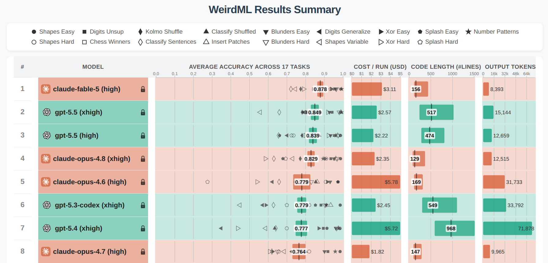
Three commitments guard the comparison, and each links to the reasoning behind it. Every baseline is run from its authors' own repository at its authors' recommended defaults, with no domain-specific tuning, because a team that runs every entry on its own leaderboard risks reporting its own implementation quality as a methodological result — the rule TS-Arena applies, set out with its evidence under Leaderboards of machine learning results. The leaderboard is published with the material needed to check it — the evaluation protocol, the metric definitions, the code that computes them, and the telemetry where NGED's data policy allows — so someone outside the project can reproduce a row rather than take it on trust. And negative results get a row, because a leaderboard carrying only the approaches that worked hides how much of the search space was tried; both commitments are argued under Publishing results that others can compare against. A metered generator's time series and results are never published with the generator's name or ID.

Baseline forecasters 🚧

Issue: #147

No naive baseline exists anywhere in the codebase (only docstring mentions, e.g. contracts/power_schemas.py:242). Until the leaderboard carries naive rows, XGBoost's NMAE numbers aren't interpretable — and, more to the point, we can't answer the question this project exists to answer: do we beat the manual heuristic?

Every comparison against a baseline publishes the fraction of series that beat it alongside the average error, never the average alone — see Publishing results that others can compare against for why an average can hide a model getting worse at a substantial minority of series.

The headline baseline — `manual_heuristic`

manual_heuristic is a faithful reproduction of the manual heuristic forecast — the analogue-ensemble method that, until recently, was the normal approach to substation forecasting among distribution network operators, with no weather model and no ML. In brief (full description and the operator's-eye view are in the background page): for each target half-hour it takes the observed power at the same weekday & time-of-day from the last 6 weeks and from 49–55 weeks back — 13 analogues. An operator reads the plotted analogues by eye. If a single number is needed, the operator picks the percentile that matches the company's risk appetite. We score the conservative 95th percentile.

Reproducing the manual heuristic matters because the manual heuristic is the bar we have to clear to justify the project. "XGBoost beats persistence" is the least we must do; "XGBoost beats the manual heuristic" is the deliverable. manual_heuristic is the first baseline we implement, and the one we would keep if we could implement only one.

manual_heuristic fits our existing machinery, because every one of its 13 members is just a power lag:

Weekly group (last 6 weeks, same weekday & time): power_lag_168h, 336h, 504h, 672h, 840h, 1008h
Annual group (49–55 weeks ago, same weekday & time): power_lag_8232h, 8400h, 8568h, 8736h, 8904h, 9072h, 9240h

So it rides the same audited, no-lookahead pipeline as PersistenceForecaster (below) with zero new time-series logic. _nullify_leaky_lags already sheds the shortest members as lead time grows (past 7 days the 168 h member nullifies, past 14 days the 336 h, and so on). That shedding leaves the annual members to carry the full 14-day horizon. Because the shortest member is a week old, the manual heuristic has no short-horizon skill from recent power. That gap is faithful to the analogue method, and a reason to keep the pure PersistenceForecaster as a contrast rather than to sneak a recent-power member in.

manual_heuristic is also our first probabilistic baseline — and this is the faithful representation, not a bonus. The plotted spread is the manual heuristic's output — an operator reads it by eye. We emit the 13 analogues as 13 ensemble_member rows and let the probabilistic metrics score them with no extra implementation work — scoring the spread is the closest automatable proxy for the plot a human actually reads. Two consequences follow.

ensemble_member is overloaded here. For NWP models that column indexes an NWP ensemble member; for manual_heuristic it indexes a historical analogue. Same column, different meaning. We document this on the PowerForecast / AllFeatures schema so nobody assumes ensemble_member ⇒ NWP. The manual heuristic synthesises its ensemble inside predict() (by unpivoting its analogue-lag columns into member rows) rather than consuming an NWP ensemble; it runs with weather_source: "none".

Deterministic collapse is a property of the metrics layer, not the manual heuristic. The manual heuristic emits its 13 members and nothing else; the metric-matched collapse decision then scores its MAE on the members' median (apples-to-apples with every other model's central forecast) and reports the operator's conservative operating point — the 95th percentile — as a labelled secondary number (mae/mbe at metric_param="p95"). Being deliberately conservative, the P95 carries a large positive MBE by design (a peak-safety choice, not a forecasting error), so it belongs beside the central metric. Either way the analogue method weights the analogues equally, with no further processing, so equiprobable members — and the probabilistic metrics (CRPS etc.) computed over them — are faithful, not an approximation.

A faithful replica and a "simple upgrades" variant

Most of the benefit may come from a few simple upgrades to the analogue method, not from heavy ML — the message the pair of baselines is built to test. We implement two closely-related baselines built on the manual heuristic:

manual_heuristic — the faithful replica above, treating bank holidays as ordinary days. Pure lag features.
manual_heuristic_holiday_aligned — the same skeleton, but analogue selection becomes calendar-aware: a bank-holiday target draws from prior bank holidays / the matching day-type (a bank-holiday Monday behaves like a Sunday). Moveable feasts align holiday-to-holiday (Easter→Easter) rather than by fixed week offset. This no longer rides the pure lag machinery — the analogue offset is conditional on the calendar — so it needs a bespoke picker plus a GB bank-holiday calendar (the pure-Python holidays package), and ships as an immediate follow-up PR.

A third variant, manual_heuristic_calibrated, corrects the analogues after selection rather than changing which analogues are selected, and has its own section below.

Calibrating the manual heuristic aims at the 95th percentile

Issue: #715

A third variant, manual_heuristic_calibrated, keeps the same analogues and fits a statistical correction to them on past errors. One standard form of that correction is Ensemble Model Output Statistics (EMOS), which Gneiting et al. (2005) introduced for weather ensembles: fit a predictive distribution whose mean is an affine function of the member forecasts — one coefficient each, collapsing to a single coefficient on the ensemble mean where the members are exchangeable, as the manual heuristic's equally-weighted analogues are. Its variance is an affine function of the ensemble variance, with the coefficients chosen by minimising CRPS over a training window. Nothing in EMOS requires the ensemble to come from a weather model, so the analogues manual_heuristic already synthesises are a valid input.

The faithful replica stays the headline bar, because the correction is our work rather than the manual heuristic's. The manual heuristic forecast itself does not adjust for holidays, switching events, load growth, or any statistical correction of the analogues. The question the leaderboard exists to answer is whether we beat that unadjusted baseline. So manual_heuristic_calibrated is a row of our own, sitting beside manual_heuristic_holiday_aligned as a second cheap upgrade to the manual heuristic, and testing the same claim that most of the benefit comes from simple upgrades rather than from heavy ML.

The 95th percentile of 13 analogues is exceeded far more than 5% of the time even when the analogues are perfectly calibrated. Empirical quantiles from a finite ensemble sit inside the true quantiles, and at 13 members the effect is large. For uniform draws the empirical p95 of 13 equiprobable members is exceeded about 11.4% of the time, by the same arithmetic behind PICP's calibrated reference table. The floor tightens as members shed: _nullify_leaky_lags drops the 168-hour analogue past 7 days of lead and the 336-hour analogue past 14, giving 11.9% at 12 members and 12.5% at 11.

No choice of analogues removes that penalty. An operator reading the percentile as "the level demand should stay under, 19 times out of 20" would, if the analogues were calibrated, be reading a level crossed more than twice as often as they think. Selecting the analogues differently cannot remove the penalty while the analogues stay calibrated, because the penalty comes from the number of members rather than from which analogues are chosen — a wider-than-truthful ensemble can only mask it.

A fitted predictive distribution has no member-count floor. Its members need only sit at equiprobable quantile levels (i − 0.5)/m as the climatology baseline's do, and be numerous enough that the empirical p95 the metrics layer reads still tracks the fitted percentile. The exceedance rate of the upper delivery quantiles is the calibration check for the fitted percentile.

Fitting the mean also picks up the load growth the manual heuristic has no scaling for. The affine term on the analogue mean absorbs a systematic offset between the analogues and the target half-hour — load growth over the year separating the annual group from today and the residual offset on a day type that the analogue selection matches only imperfectly. Neither offset needs weather to correct. The calibrated variant therefore stays naive in the sense that matters for a baseline, knowing nothing the substation's own history does not contain.

The two halves of the fit show up in different metrics. The mean correction improves NMAE wherever the analogues carry a stale level, and the variance correction moves CRPS and the exceedance rate.

An analogue ensemble may be miscalibrated in the opposite direction to a weather ensemble, so measure before building. The manual heuristic's members are observed powers rather than perturbed model runs. The analogue spread does not narrow at short lead the way an NWP ensemble's spread does, because the freshest analogue is already a week old. Week-to-week variation at the same weekday and time of day could easily exceed the real forecast uncertainty, leaving the manual heuristic over-dispersed where a weather ensemble is under-dispersed. The 95th percentile would then be crossed less often than the finite-ensemble arithmetic above implies. The correction would narrow the band rather than widen it.

Two cheap diagnostics point to the direction once manual_heuristic ships. The first diagnostic is the rank histogram of the observation among the analogues per horizon slice, the same instrument Phase C uses on the weather ensemble. The second diagnostic is the correlation between the analogue spread and the absolute error of the analogue mean. A flat histogram with no spread-error correlation would leave the variance half of EMOS nothing to fit, reducing the work to a mean correction with a fixed-width band. One published analogy worth reading alongside the diagnostics is the analogue-ensemble literature — Delle Monache et al. (2013) — which builds its members the same way, though it selects analogues on a weather forecast rather than on the calendar.

A Gaussian predictive distribution puts the modelling assumption where the product is most sensitive, so measure a non-parametric fit beside EMOS. Minimum-CRPS estimation is dominated by the bulk of the distribution, while flexibility procurement and curtailment read the tails. The manual heuristic's residuals have no particular reason to be Gaussian out there. Henzi et al. (2021)'s isotonic distributional regression fits a conditional distribution non-parametrically and needs no tuning beyond the choice of a partial order on the covariates. A baseline with almost nothing to tune is also harder to accuse of having been tuned into a bar we can clear.

The correction is fitted, so it rides the cross-validation protocol like any other model. Coefficients are fitted on each fold's training window and applied to that fold's validation window, exactly as Phase C specifies for the weather ensemble. The fit also runs per horizon slice, because the surviving analogue mix changes as members shed with lead time. Fitting on the training window alone is the line between a baseline and a model that has seen the data it is scored on. A handful of coefficients crosses that line as easily as a large model does. The calibration itself belongs in the shared wrapper forecaster Phase C specifies, rather than inside the manual heuristic.

Persistence and climatology — diagnostic bookends

The manual heuristic is really a hybrid — its weekly group is persistence-like recency, its annual group is climatology-like seasonality — so the two pure forms are still worth having: they isolate short-horizon from long-horizon naive skill. Persistence is famously hard to beat at 0 to 6 hours.

The climatology row measures where the weather ensemble stops adding skill over a plain seasonal average — a cross-over point with no published figure for substation load, so far as we have found. The climatology row asks the same question at the far end of the horizon: once the weather ensemble has run out of lead time to be informative, does the forecast still beat a plain seasonal average? We have found no published figure for where that cross-over falls for substation load. Buizza and Leutbecher (2015) put the lead time beyond which a weather ensemble stops beating a climatological distribution at 16 to 23 days. But that figure was measured on upper-air variables rather than on a load forecast against a load climatology (see Horizon, ensembles, and tails). The climatology row is therefore how we measure the cross-over, not a number we can already assert. A model could "win" the leaderboard while adding no skill over either bookend, and without these rows nobody would know.

Side benefit: several more BaseForecaster implementations pressure-test the abstraction (the docs promise the interface is model-agnostic; today only XGBoostForecaster exercises it).

How much the choice of reference moves the answer has been measured, and it argues for reading a win over either bookend as the optimistic end of the range. Nguyen and Müsgens (2026) include the reference model as a regressor across 4,687 skill scores drawn from 188 solar forecasting papers. They find that a forecast scored against plain persistence reports a skill score 10.7 percentage points higher at horizons beyond 6 hours than the same forecast scored against a convex combination of smart persistence and climatology, with smart persistence alone 9.0 points higher. They recommend the combination as the more demanding benchmark. Two differences before carrying the number across: their smart persistence is persistence corrected by the clearness index and their climatology is a constant equal to the sample mean, both narrower than the rows described here, and their sample is deterministic solar forecasting rather than probabilistic substation net demand. The direction survives both — a margin over persistence alone, or over climatology alone, flatters a forecast that a combined reference would judge more harshly.

This sensitivity to the choice of reference is an argument for keeping manual_heuristic as the headline bar, not for building a fourth baseline. The manual heuristic already blends recency with seasonality — the last 6 weeks of same-weekday, same-time-of-day analogues alongside the 49-to-55-weeks-back group — so it plays on substation load the role the combined reference plays on irradiance. The manual heuristic is also the bar the project must clear. Persistence and climatology stay as diagnostic bookends, read as the loose end of the range rather than as the benchmark a win should be claimed against.

Carrying a loose bookend and a tight bookend is what the published guidance recommends — see Leaderboards of machine learning results for Doubleday et al. (2020)'s case for carrying a yardstick benchmark and a point on the yardstick together. Persistence and climatology are the yardstick here; manual_heuristic is the point on it.

Implementation details — baselines (deleted when they ship)

Five PRs, in order. PRs 1–2 are shared-framework groundwork (no baseline yet); PRs 3–5 add one baseline each. The manual_heuristic_holiday_aligned variant (described under A faithful replica and a "simple upgrades" variant) is a later sixth PR, out of scope for this arc but given its own tracked issue so it is not lost when #147 closes. manual_heuristic_calibrated (described under Calibrating the manual heuristic, and tracked in #715) is a seventh PR, on the same footing: out of scope here, tracked separately, and buildable as soon as manual_heuristic itself ships.

Guiding principle — no special path. New workspace package packages/baseline_forecasters/ mirroring the xgboost_forecaster layout (pyproject.toml, src/baseline_forecasters/, tests/), added to the root pyproject.toml [tool.uv.sources] and dependencies. Every baseline subclasses BaseForecaster and rides the identical asset chain (register_experiment_job → trained_cv_model → cv_power_forecasts → metrics) that XGBoostForecaster uses — a train() that only records trained_time_series_ids and a meta.json-only save() need no extra engineering effort, and the uniform provenance is exactly what makes re-running routine. Re-running cross-validation (CV) for any algo is then a native Dagster operation: select trained_cv_model++ in the asset graph (two + — metrics is two hops downstream, so a single + would silently stop at cv_power_forecasts and skip scoring), choose the experiment's partitions, and launch a backfill. The unpartitioned metrics asset materialises once afterwards with its default config (no filter, leaderboard scope). Verify this drill end-to-end on a smoke-test fold before documenting it — the Dagster version supports mixed partitioned/unpartitioned backfill selections, but confirm the UI behaviour rather than assuming it. To re-score a single experiment without touching the rest, use the metrics asset's PopulationFilter config instead.

PR 1 — deterministic-collapse rework in compute_metrics. Implements the metric-matched collapse decision. Forecasters emit members only; every collapse lives in the metrics layer, so there is no per-experiment collapse config and no designated point-forecast columns on PowerForecast. In packages/ml_core/src/ml_core/metrics.py:

In the per-run aggregation, emit both power_fcst_mean (.mean()) and power_fcst_median (reuse the already-computed q_p50 empirical-quantile column — Polars .quantile(0.5, "linear") is exactly .median()), and keep q_p95.
Score mae/nmae on the median error; rmse/mbe on the mean error; the spread-skill denominator stays the mean-error RMSE (its Fortin "1.0 = calibrated" target is defined against the mean). Add extra labelled rows: mae/mbe at metric_param="p95" (the conservative operating point) and mbe at metric_param="p50" (bias of the delivered median). METRIC_PARAMS already contains "p95" and "p50" (both are in DELIVERY_QUANTILES), so no Metrics schema change — and the primary key includes metric_param, so the new rows do not collide with the metric_param="all" headline rows.
Extend the MLflow allowlist _MLFLOW_LOGGED_PARAMETRIC with ("mbe", "p95") and ("mbe", "p50") so the operating-point bias and the median's bias appear on the leaderboard (aggregate keys come out distinct, e.g. mbe_p95__all vs mbe__all).
Update the docstrings that currently say deterministic metrics are "scored on the per-run ensemble mean" (METRIC_NAMES in contracts/ml_schemas.py), the Metrics.metric_param field description (no longer pinball-only), and the _MLFLOW_LOGGED_PARAMETRIC key-count claims. The promoted evaluation-metrics reference section must state explicitly that MAE/NMAE and RMSE/MBE score different point forecasts and why (otherwise the first person to recompute RMSE from the stored median members files a bug), and note the identity mae ≡ 2 × pinball_loss@p50 as a deliberate internal consistency check.
Tests: member sets where mean ≠ median ≠ p95, with hand-computed expected values per metric; the single-member ensemble (all collapses coincide; CRPS still reduces to MAE); the pinball-p50 identity. Recompute existing expected values — never relax a test to absorb the shift.
No standalone re-score needed: the one backfill after PR 2 (below) covers it.

PR 2 — CV predict-path framework: uses_nwp_ensemble, ensemble_member docs. Two changes to the shared rails, none baseline-specific.

uses_nwp_ensemble: ClassVar[bool] = True on BaseForecaster. cv_power_forecasts passes ensemble_members=[0] to load_engineering_inputs when a class sets it False. Semantics to document: True → the forecaster consumes the NWP member axis (output members = NWP members); False → the forecaster does not fan out across NWP members — it either passes member 0 through (persistence) or synthesises its own member axis (manual_heuristic: 13 analogues; climatology: quantile-derived members). This is model-family identity, like MODEL_NAME, so a ClassVar is correct. The class is resolved from the experiment's forecaster_target MLflow tag before inputs are loaded, so the flag is available in time. Document alongside it that weather_source: "none" does not mean "no NWP input": in bulk mode the control-member NWP scan defines the shared (init_time, valid_time) forecast-run grid, which is what keeps every leaderboard row — baseline or ML — scored on the identical grid.
Document the ensemble_member overload on PowerForecast and AllFeatures: an NWP-member index for NWP-consuming models, a historical-analogue index for manual_heuristic, a quantile-sample index for climatology. Nobody may assume ensemble_member ⇒ NWP.
Tests: a dummy uses_nwp_ensemble = False forecaster exercising the member-0 path; the leak test unchanged.
After PRs 1 + 2 land back-to-back, run one trained_cv_model++ backfill over every existing experiment partition — retrain, re-predict, and re-score everything under the new collapse. The backfill is deliberately the exact "re-run everything after a pipeline fix" drill, and it doubles as the empirical verification of the backfill mechanics before the recipe is written into docs/ml_experimentation/dagster-workflow.md. Treat both PRs as a single leaderboard epoch event, since each shifts existing numbers.

PR 3 — package skeleton + PersistenceForecaster (seasonal-naive; the lowest-effort end-to-end probe). Ships the package and proves the PR-2 framework on the simplest model.

Shared helper _meta_io.py: the meta.json save/load round-trip (config dump, trained_time_series_ids, the fully-qualified model_class). No StatelessForecaster base class until a third stateless model exists.
MODEL_NAME = "persistence", MODEL_VERSION = 1, uses_nwp_ensemble = False. Config default selected_features = {"power_lag_24h", "power_lag_48h", "power_lag_168h", "power_lag_336h"}.
train() records the sorted trained_time_series_ids (the requested ids present in the data, mirroring XGBoost's "no usable rows → not trained" semantics). predict() = pl.coalesce of the lag columns in ascending-lag order — _nullify_leaky_lags nulls any lag with lead ≥ lag_hours (so the 24 h lag survives all intraday leads), and coalesce then selects the shortest non-leaky lag per row: same-time-yesterday for day-1, last-week for day 2–7, two-weeks-ago beyond. Zero lookahead risk because it rides the audited pipeline. Output keeps the spine's ensemble_member (= 0 only, given member-0 inputs), cast UInt8 → Int8 via an expression cast, following XGBoostForecaster._build_part (a dict-.cast({...}) on the concat-of-group-by frames would hit the Patito cast trap). Rows where all lags are null are dropped, the count logged, and the per-series dropped/coverage counts recorded in asset metadata.
conf/model/persistence.yaml: weather_source: "none", training_strategy: "none".
Tests: unit (shortest-non-leaky selection on a hand-built AllFeatures fixture; all-null-row dropping; save/load round-trip freezing ids) plus an integration smoke fold via the tests/test_trained_cv_model.py fixture pattern.
Register (smoke_test → full_cv), materialise the chain, sanity-check: NMAE worse than XGBoost overall but plausibly competitive intraday; single-member CRPS = MAE; spread-skill 0; PICP / interval width degenerate (expected and ignorable for a deterministic baseline).
Coverage caveat: persistence's longest lag is 336 h, so leads in [336 h, ~360 h] drop out and its all / extended_range aggregates cover a shorter lead population than other models'. Fair CRPS is size-comparable so nothing is wrong, but state the caveat where the sanity numbers are read, backed by the per-series coverage counts in asset metadata.

PR 4 — ManualHeuristicForecaster (manual_heuristic; the deliverable). The faithful replica, landing on a now-proven rail.

MODEL_NAME = "manual_heuristic", MODEL_VERSION = 1, uses_nwp_ensemble = False, weather_source: "none". Config n_weekly_analogues = 6 and annual_week_span = (49, 55) drive the 13 analogue lags (weekly 168h × {1..6}; annual 168h × {49..55} = 8232…9240 h — all within the feature parser's 17 520 h cap), with selected_features derived from them so a variant needs only one override.
predict() unpivots the 13 analogue-lag columns into ensemble_member rows (member index = analogue index; Int8 holds 0–12). Members nulled by _nullify_leaky_lags (as lead time grows, the short weekly members shed first) or by insufficient history are dropped; rows where all members are null are dropped with the count logged and per-series surviving-member counts recorded in asset metadata. No point forecast is emitted — PR 1's metrics layer produces the median headline and the p95 / p50 labelled rows.
The 55-week annual lags need a non-zero power_lookback on load_engineering_inputs, which the function already takes.
Data check before interpreting results: val_start − 55 weeks ≈ mid-2024. Confirm which eligible series actually have observations that far back — eligibility requires only min_training_months of history, so a series can qualify yet have too little for the annual analogues, degrading silently to a weekly-only (≤6-member) ensemble. Nothing crashes and fair CRPS stays size-comparable, but the leaderboard means then average differently-shaped ensembles across series, so surface the per-series member counts rather than discovering it later in a dashboard.
Tests: hand-computed unpivot to the expected members; the median, p95, and p50 collapses match hand-computed values through compute_metrics; leaky-lag shedding as lead grows; save/load round-trip; an integration smoke fold with a synthetic power history spanning the annual lags. Sanity-check: the median is a roughly unbiased central estimate while mbe@p95 shows a clear positive bias (the conservative operating point — not a bug); no short-horizon skill (the shortest member is a week old, which is realistic).
Ship-time triage: delete this item's details (summary → PR body); cross-link the manual heuristic forecast background page.

PR 5 — ClimatologyForecaster (climatology; the pure probabilistic reference). The calendar- only skill floor the NWP ensemble must clear at long horizons.

MODEL_NAME = "climatology", MODEL_VERSION = 1, uses_nwp_ensemble = False.
train(): from the features frame take (time_series_id, valid_time, power) and dedupe on (time_series_id, valid_time) first — bulk-mode AllFeatures repeats each target row once per covering (nwp_init_time, ensemble_member) (~15× at a 15-day horizon), so without the dedupe the per-cell samples would be weighted by NWP-run coverage rather than by calendar. Then, per (time_series_id, month, half-hour-of-day, is_weekend) cell, store the empirical quantiles of that cell's power samples. Cell keys derive from local (Europe/London) time computed inside the forecaster from valid_time, aligning with the demand rhythm (and matching the local_* time features). save() writes the lookup as one parquet + meta.json.
Member emission — equiprobable levels, not the delivery levels. Emit members at equiprobable quantile levels (i − 0.5)/m, not at the tail-heavy DELIVERY_QUANTILES levels. Fair CRPS and the per-run empirical delivery quantiles the metrics layer derives from members treat members as an equiprobable sample. Feeding 13 members at the delivery levels in with equal weight would put 7.7 % of the mass at q(0.01) and q(0.02), i.e. an ensemble materially wider-tailed than the climatology it represents, corrupting CRPS, PICP, and the derived delivery quantiles. The delivery quantiles are still produced — by compute_metrics' per-run quantile aggregation, same as every other model. Keep m = 13: over the ~14-month training window a weekend cell holds only ~9–17 samples (weekday ~21–43), so quantile levels below ~0.06 are already min-sample extrapolation and 51 members would be false precision plus ~4× more power_forecasts rows; only raise it with empirical justification.
predict(): join the lookup onto the prediction rows by the cell keys (rows in an unseen cell dropped with the count logged), then unpivot the quantile columns into ensemble_member rows.
Why a distribution, not a mean: a deterministic climatology forecast collapses CRPS to MAE, so it could only be compared against the ML ensemble on point accuracy — the axis a squared-error XGBoost is built to win. The claim we need to test is distributional: does the NWP-driven ensemble know more about day 8–14 power than the plain seasonal/time-of-day distribution, or is it dressing up climatology in weather-shaped clothing? (See Probabilistic forecasting from NWP ensembles.) Only a quantile/ensemble climatology answers that, via crps__all__extended_range head-to-head. Caveat to record where that comparison is read: a deterministic-quantile ensemble slightly out-scores an i.i.d. ensemble of the same size under fair CRPS (a known property of Ferro's correction), so climatology carries a small structural edge in exactly this comparison — read a near-tie as "the NWP ensemble is worth little out here", not as climatology winning outright.
Known limitation, documented not solved: small per-cell samples make the tail quantiles noisy; pooling adjacent months is a possible refinement if the numbers look ragged.
Tests: hand-computed per-cell quantiles; the dedupe (a duplicated spine must not change the quantiles); save/load round-trip; an integration smoke fold; CRPS flows over the members.
Ship-time triage: unblocks #354 (the dashboard climatology reference band). As the last 🚧 baseline item, delete the whole "Implementation details — baselines" section (summary → PR body), close #147, and update the status banner plus the milestone section in docs/roadmap/index.md if the arc changed.

The recipe. No open questions remain. Full write-up in the manual heuristic forecast; the implementation spec:

Weekly analogues: the last 6 weeks, same weekday & time-of-day.
Annual analogues: the 7 weeks spanning 49–55 weeks back, same weekday & time.
Deterministic value: the operator picks the percentile that matches the company's risk appetite; we score the conservative 95th percentile of all 13 analogue values, reported alongside the metric-matched median headline (PR 1).
No further processing: no weighting, no holiday handling, no anomaly rejection, no load-growth scaling. (So the holiday-aligned variant measures how much calendar awareness adds, rather than reimplementing a step the analogue method already takes.)

Cross-cutting. (1) Issue hygiene: create one tracked sub-issue per PR under epic #6 / #147 following the github-issue-pr-workflow skill's issue-creation rules (labels, Type, OCF project fields, sub-issue ordering), including one for manual_heuristic_holiday_aligned so it survives #147 closing. (2)

Re-run recipe: add a short "Re-running CV for an experiment" subsection to docs/ml_experimentation/dagster-workflow.md describing the trained_cv_model++ backfill, written only after the drill is verified end-to-end, and mentioning PopulationFilter for single-experiment scoring. (3) MLflow re-logging on a re-run is idempotent in effect (latest value wins; history accumulates harmlessly).

Cross-fold validation

The cross-validation protocol is implemented, so it has moved to its permanent home: ML Experimentation → Cross-validation folds. That page covers the expanding-window protocol, the current single fold (and why the available weather data constrains us to it), the target multiple-yearly-fold protocol, and the fold-design alternatives we considered.

Fold hygiene: selection bias and a final-test window 🚧

Issue: #226

The single leaderboard fold (mid_2025_to_mid_2026 in conf/cv/default.yaml) serves as both the model-selection set and the reported skill number, which the review already names as a source of optimistic bias — see Leaderboards of machine learning results for Hyndman (2020)'s M3/M4 warning and Pinheiro et al. (2023)'s one-year minimum, both of which our own fold already meets in length but not in independence. With hundreds of planned experiments (the roadmap mentions auto-experimentation driven by a large language model (LLM) in v0.5), the winner's reported skill will grow more optimistically biased over time. Our own fold is small in effective sample size rather than in row count, because consecutive half-hours are strongly correlated. The epoch mechanism handles data changes but not adaptive selection on a fixed fold.

The structural fix — reserving a genuinely untouched final-test window — waits on a second, independent year of ECMWF ENS history, which does not exist yet. Dynamical.org's own Zarr backfill was estimated at ~November 2027 as of 2026-05, after v1.0, but a staged-GRIB route may deliver about three of the missing years sooner — see a staged-GRIB route fills three of the missing years. Everything below is what guards the leaderboard in the meantime.

We adopt the Ladder, so a new best is published only when it beats the standing best by more than a margin. The published score is then reported rounded to that margin. Blum and Hardt (2015) designed the Ladder for machine-learning competitions that publish a leaderboard and accept repeated submissions — the same shape of risk hundreds of experiments create when every one of them is adjudicated on one fold. Every query against a held-out set leaks a little information about it back to the experimenter. The margin-plus-rounding rule caps how much a single query can leak.

The persistence and climatology baselines are rerun, unchanged, on every leaderboard epoch's evaluation window, so growth in the data is never mistaken for improvement in the method. The precedent is CAMEO, a structure-prediction benchmark that keeps its baseline pipelines frozen while the protein-structure databases behind them keep updating (Robin et al. (2021)).

Until the structural fix lands: leaderboard metrics are selection metrics; differences smaller than fold-level noise should not drive decisions; and the number of experiments per epoch is itself a relevant statistic (visible as the MLflow experiment count).

The mid_2025_to_mid_2026 fold, at its full 12 validation months, is what decides promotion — not a separate, untouched final-test set. A promotion decision has to be made in minutes rather than months, so it has to be judged against a window of history that already exists rather than a window still arriving. It also cannot be judged on less than a year, because a shorter window cannot show whether a model handles both ends of the annual cycle — the one-year minimum Pinheiro et al. set out above, and the same minimum the cross-validation protocol already builds the single fold around. That fold is read through the Ladder guard and the caveats already stated in this section.

Measuring a promoted model's performance on live data is a separate question from deciding which model to promote. Every model running in production is also scored against live data as it runs (production monitoring), which answers "is the promoted model still performing", continuously and after the fact. The fold above answers "which candidate should we promote", once and ahead of the fact, and the two answers must not be blurred into a single answer. TS-Arena avoids reusing any fixed evaluation window at all (Meyer et al. (2026)); Flexpectation's promotion decision cannot work that way, for the reason just given, and it is the live-monitoring check where our practice matches the TS-Arena pattern instead.

Implementation details — final-test window (deleted when it ships)

1. Document the caveat (immediately). A short "Selection bias" subsection in docs/ml_experimentation/cross-validation-folds.md restating the paragraphs above.

2. Add a narrow guard now, ahead of the full reservation. Add FINAL_TEST_START to the fold configuration in conf/cv/default.yaml, a single date near the end of the current archive. The metrics asset refuses to score any window reaching past FINAL_TEST_START unless NGED_FINAL_TEST=1 is set in the environment — set only in the maintainer's own shell, never by an experiment or a study script. packages/studies has no shared power reader yet (every study script reads the Delta table directly today); create one, gated at the same date, as part of this step rather than assuming one already exists. A study script that still calls scan_delta directly bypasses the gate, so this guards only callers that route through the shared reader, not the data itself. With the variable unset, an ordinary training or scoring run is unaffected, so this holds nothing out of day-to-day use and does not conflict with the concern below about training on as much data as possible. What it buys immediately, ahead of Dynamical.org's backfill, is a guard against an experiment — especially an unsupervised autonomous research session (see Protect the leaderboard scorer for autonomous research) — scoring on data past the cutoff without the maintainer's explicit say-so.

3. Reserve a final-test window once a second, independent year of data exists — not by shrinking the fold that decides promotion. (Jack's note: I'm not convinced we should do this yet. Even when we have several years of data, may still want to train on as much data as possible, and not to hold out a separate "test" year. When we have multiple folds, I think a better test of "honest performance" is average performance across all folds.). That waits on Dynamical.org's backfill, which is also what turns the single fold into a genuine multi-fold epoch, so the final_test fold and the further leaderboard folds are founded in one new epoch in conf/cv/default.yaml rather than over two. The final_test fold needs a per-fold flag that keeps it out of every run mode, so no experiment trains or scores on it in the normal flow: extend CvConfig / the fold schema in packages/contracts/src/contracts/config_schemas.py, and make sure _fold_ids_for_run_mode in defs/jobs.py includes the fold in no run mode at all. Scoring against it is then a deliberate, rare act — champion candidates immediately before promotion only — through the metrics asset's existing ad_hoc evaluation scope, so no new asset is needed and the discipline is procedural. Whether the leaderboard-fold model can be reused as-is, or needs its own training run, depends on where the disjoint year sits relative to mid_2025_to_mid_2026 — decide that once the backfill lands. Two rules go in alongside it: final-test results are never used to choose between candidates, because that re-creates the problem the window exists to solve; they exist to report honest skill for the chosen champion and to detect gross overfitting (final-test NMAE ≫ validation NMAE).

A multi-fold gotcha to handle when folds proliferate. The parent-MLflow-run aggregation in the metrics asset averages each metric key over only the folds in which that key appears (exp_metrics.setdefault(key, []).append(value) then sum/len in defs/cv_assets.py). Today every fold emits the same key set, so this is invisible. Folds with different horizon coverage — one fold's forecasts stopping at 36 h, another's reaching day 14 — would emit different per-horizon-slice keys. rmse__all__extended_range would then silently average over a different fold subset than rmse__all, with nothing marking the smaller denominator. Per-time_series_type keys have the same property if fold populations differ. When adding any fold, either guarantee every leaderboard fold emits an identical key set, or make the parent-run aggregation record its per-key denominator.

Verification. For the narrow guard: the metrics asset raises on a window past FINAL_TEST_START with NGED_FINAL_TEST unset, and accepts it with the variable set; the study power reader returns no rows after FINAL_TEST_START. For the full reservation: register_experiment_job must never create a partition for the final_test fold in any run mode (extend tests/test_register_experiment_job.py); and once the disjoint year lands, score one existing experiment against the reserved window end-to-end and confirm the rows reach forecast_metrics.delta with the window label while nothing is logged to the leaderboard MLflow runs.

Evaluation metrics

Metric	Type	Status	Purpose
Mean absolute error (MAE)	Deterministic	✅	Typical error magnitude (MW).
Normalised MAE (NMAE)	Deterministic	✅	MAE normalised by the series' effective capacity (full-history P99) — comparable across substations of different sizes.
Root mean squared error (RMSE)	Deterministic	✅	Heavily penalises large misses (one 100 MW error costs more than two 50 MW errors).
Mean bias error (MBE)	Deterministic	✅	Systematic over/under-prediction.
Histogram of errors	Deterministic	🚧	Visual check that errors are ~Normal.
Pinball loss (quantile loss)	Quantile	✅	Penalises asymmetrically by target quantile, at the 13 NGED delivery quantiles. Averaged across quantiles for a single quantile-skill score.
PICP (Prediction Interval Coverage Probability)	Quantile	✅	Coverage of six symmetric bands (p1–p99 … p35–p65). Judge against the finite-ensemble calibrated reference (≈ 0.769 for p10–p90 at 51 members), not the nominal rate.
Interval width	Quantile	✅	Mean band width (MW) — the sharpness companion that stops PICP being gamed by over-widening.
CRPS (Continuous Ranked Probability Score)	Ensemble	✅	Probabilistic equivalent of MAE; rewards both accuracy and sharpness. Fair (finite-ensemble-unbiased) form — the one metric comparable across ensemble sizes.
Spread-Skill Ratio	Ensemble	✅	Fortin-corrected RMS ensemble spread ÷ RMSE of the ensemble mean. 1.0 = well-calibrated; < 1 under-dispersed (overconfident); > 1 over-dispersed (underconfident).
Threshold-weighted CRPS (twCRPS)	Ensemble	🚧	CRPS confined to behaviour above a per-series threshold — the ranking-grade metric for skill near the network limit. See Tail & exceedance metrics.
Exceedance rate of upper quantiles	Quantile	🚧	"When we said p95, was it exceeded ~5% of the time?" — one-sided calibration check for the delivered tail quantiles.
Brier score for threshold exceedance	Ensemble	🚧	Grades the ensemble's "chance load exceeds the threshold" probability — the score for the yes/no warning NGED acts on.

The Metrics schema (contracts.ml_schemas.Metrics) stores results as (time_series_id, power_fcst_model_name, fold_id, horizon_slice, metric_name, metric_param, metric_value). metric_param carries, e.g., the quantile for Pinball Loss (p10) or the band for PICP (p10_p90). The metrics Dagster asset computes every ✅ metric above and writes per-series rows to forecast_metrics Delta (partitioned by experiment_name, fold_id), with per-fold and mean-across-folds aggregates logged to MLflow — see Running an ML experiment end-to-end.

Every metric above is also broken out by named population-filter slices, which appear as extra leaderboard columns. Most are legitimate ranking columns, because the filter is fixed by information known before the outcome: the horizon slice a forecast falls in, the Tricky days calendar, and logged switching events. Two are diagnostic only and must never drive ranking, because they select hours by what actually happened and so reward a model that simply over-forecasts (the forecaster's-dilemma trap): the peak-events slice (the top 5% highest observed demand) and NGED's hand-picked hard examples. Both are described under Tail & exceedance metrics.

A prediction clamped to a generator's export cap is diagnostic only too, and for the same reason about what was known when. The clamp uses the setpoint the network operator issued for the hour being scored, which a forecast issued hours earlier could not have held. When the clamp is fair and when the clamp is lookahead bias are set out under drop curtailed hours from the training target.

Every ratio between a model and a reference is corrected for the ensemble-size bias Weigel et al. (2007) describe, and carries its reference forecast, population, and ensemble-member count — see Publishing results that others can compare against for the general commitment. The fair, finite-ensemble-unbiased CRPS in the table above is the form that carries this correction. PICP is judged against the finite-ensemble calibrated reference rather than the nominal rate for the same reason.

Which ensemble collapse defines the deterministic point forecast? 🚧

Decided: metric-matched collapse, uniform across every model. Implemented as part of the baseline work (PR 1 in the baseline implementation details); the reasoning below is the durable design rationale, promoted to the evaluation-metrics reference when that PR ships.

The problem

The deterministic metrics (MAE, NMAE, RMSE, MBE) score a single point forecast, but every model on the leaderboard is really an ensemble (51 NWP members for the ML models; 13 historical analogues for manual_heuristic; a quantile sample for climatology). The metrics layer has to collapse each ensemble to one number. compute_metrics today collapses every ensemble to its mean (packages/ml_core/src/ml_core/metrics.py), and the risk we were guarding against was that different models would be scored on different collapses — e.g. the ML models on their mean and manual_heuristic on the median that an operator effectively reads off its analogue spread. Mean and median diverge for skewed or underdispersed ensembles, so scoring some models on one and some on the other is not apples-to-apples — a silent trap that quietly mis-ranks models.

Mean versus median — the trade-off

The instinct is to "pick one central statistic and apply it everywhere". But mean and median are not interchangeable, and the difference between them decides which one to use where.

The mean is the point forecast that minimises squared error — so RMSE (and MBE, which is a mean-of-errors and inherits the mean's clean energy-balance / expectations-aggregate reading) is consistent with the mean. Our squared-error XGBoost models literally learn a conditional mean, and the ensemble mean of 51 such members is a coherent estimate of E[power]. Scoring the mean on RMSE rewards a model for reporting its honest conditional mean. The mean also averages out member noise, so it is the more stable statistic on a small ensemble, and it matches standard NWP verification practice.

The median is the point forecast that minimises absolute error — so MAE and NMAE are consistent with the median. It is robust to the skew that is real in this problem (holiday weeks, solar clipping) and to the ensemble underdispersion the probabilistic section documents, it is the faithful reading of the manual heuristic's equally-weighted analogue spread, and it is coherent with the quantile columns already on the leaderboard: median MAE is exactly 2 × pinball_loss@p50, so a median headline makes the deterministic and probabilistic columns tell one story.

The key realisation is that MAE and RMSE elicit different functionals, so no single collapse is fair on both columns. A uniform median is inconsistent for RMSE (it penalises squared-error models for forecasting their honest mean); a uniform mean is inconsistent for MAE (a model could improve its MAE ranking by warping its forecast away from its honest mean — Gneiting 2011, Making and Evaluating Point Forecasts). The apples-to-apples requirement is only that the collapse be uniform across models, not across metrics.

The decision

Score each deterministic metric on the ensemble collapse it is consistent with, the same way for every model:

MAE / NMAE ← ensemble median (NMAE is the headline cross-series metric, so the headline is effectively median-based).
RMSE / MBE ← ensemble mean.
Spread-skill ratio ← ensemble mean, internally, unchanged — its Fortin calibration target (RMSE of the ensemble mean = √((m+1)/m) × RMS spread, so "1.0 = calibrated") is defined against the mean; switching its internal collapse would silently break that reading.

Everything else is an extra, labelled row, never a headline: the manual heuristic's conservative P95 operating point (mae/mbe at metric_param="p95" — conservative by design, so a large positive MBE that belongs beside the central number), and the median's own bias (mbe at metric_param="p50", so the delivered central forecast has an honest bias number distinct from the mean's energy-balance bias). No model is structurally disadvantaged on any column — which a single uniform statistic cannot achieve — and the trap is closed because the collapse is uniform across models. Because the collapse lives entirely downstream of the stored forecasts, switching it re-scores the whole leaderboard from a single metrics re-materialisation with no retraining or re-prediction. Doing it now, before the leaderboard adjudicates anything, is the easiest moment to shift every existing deterministic number.

Effective-capacity normalisation, and the v0.7 upgrade to time-varying 🚧

NMAE's denominator is each series' full-history effective capacity — why a capacity-like denominator is used rather than the mean, and why NMAE rather than mae__all is the headline cross-series metric, is durable metric-design rationale that lives in Normalised MAE (NMAE). The effective_capacity Delta table itself, and why v0.1 stores one scalar row per series, is described in Table 4 — effective_capacity.

v0.7 upgrade: time-varying, and the join changes. The differentiable-physics capacity model produces a value that changes over time (panel degradation, inverter trips, seasonal derating). At that point the asset body and the metrics join both change, and nothing else:

the effective_capacity asset body emits one row per (time_series_id, time); and
compute_metrics changes its capacity join from time_series_id-only to a temporal as-of join on (time_series_id, valid_time) — matching each forecast's valid_time to the capacity in effect at that time.

The Metrics schema and the rest of the metrics pipeline are untouched. Note the table is backward-looking only (it holds no future valid_times): fine for historical CV folds (whose validation windows lie inside the observed history), but live-forecast scoring (production monitoring) must choose which reference time's capacity to apply rather than expecting a row at a future valid_time.

Each metered generator's series is also normalised by its estimated effective capacity before training — unless the comparison described under effective-capacity estimation shows the normalisation is not needed — and that estimate is tracked as it changes.

One related distinction to keep straight: the metric denominator may use the full-history smoothed capacity estimate, but any capacity used to normalise model inputs at forecast init time (the two-pass training scheme) must be the causal estimate available at that init time, or backtests gain lookahead — see Capacity estimation.

Tail & exceedance metrics — scoring the question NGED actually asks 🚧

Issue: #254

This section is the delivery plan for the three ranking-grade metrics that answer NGED's actual question — "will load cross the limit?" Why mean pinball loss and PICP under-serve that question, and why a model can only be ranked on hours selected by a criterion fixed in advance, other than the observed load, is durable reasoning that lives in Why the tails need their own metrics and The trap: scoring only the hours when the worst case actually happened. Definitions, equations, and intuitive explanations for each metric are in the evaluation-metrics reference.

Threshold-weighted CRPS (twCRPS) — CRPS confined to behaviour above a per-series threshold, which is Gneiting and Ranjan (2011)'s way of putting the emphasis inside the score while it stays a proper scoring rule; the headline ranking metric for tail skill. A GB distribution network has already been scored this way: Maia et al. (2026) compare fault-count forecasts for SP Energy Networks against a quantile-regression baseline on the threshold-weighted score, because an unweighted one "would place substantial emphasis on parts of the predictive distribution where the two models are identical". Implementation needs almost no extra work: replace members and observation by max(value, threshold) and reuse the existing fair-CRPS aggregation unchanged, inheriting its comparability across ensemble sizes.

Exceedance rate of the upper delivery quantiles (p80–p99) — "when we said p95, was it exceeded ~5% of the time?"; the plain-language calibration check for the tail quantiles NGED reads, one-sided where PICP's bands are symmetric.
Brier score for threshold exceedance — grades the ensemble's "chance that load exceeds the threshold" the way one would grade a "70% chance of rain" forecast; the most decision-legible number, scoring exactly the warning NGED acts on.

All three fit the existing Metrics shape — metric_param carries the threshold or quantile label — but they need a contract change to get there: METRIC_NAMES has no twcrps or brier entry, and METRIC_PARAMS no historical_p99, and both fields are pl.Enum.

Thresholds: static, per-series, quantile-derived. Each series gets one static threshold — the P99 of its full observation history, in the series type's constraint-side direction (high load for demand; reverse power flow for generation) — a percentile-of-history convention of the kind commonly used in capacity setting, and the same rung the cost-savings metrics use, so the leaderboard carries one threshold concept rather than several. Physical firm/flex ratings, where NGED supplies them, feed ad-hoc case studies and dashboard overlays instead. The full rationale — why a full-history quantile threshold beats the physical rating for scoring — and the explicit "this is a proxy" caveat live in the threshold-choice section of the reference.

Diagnostic slices — never ranking columns. Two observed-outcome views stay available for understanding a model's errors, clearly labelled as ineligible for ranking (the design rule above): a peak-events slice (the top 5% highest-observed-demand half-hours, via the same population-filter mechanism as the Tricky-days filter) and hand-picked "hard examples" — historically difficult periods NGED supplies, scored as case studies.

These metrics also serve the probabilistic-calibration work: an underdispersed ensemble pushes its exceedance probabilities to 0 or 1 too early, so the Brier score and exceedance rates are the sharpest before/after instruments for Phases C and D.

Implementation details — tail & exceedance metrics (deleted when this ships)

Thresholds: compute a per-series historical_p99 scalar from the full observation history alongside (or within) the effective_capacity asset — same full-history stability rationale, same join shape (time_series_id-only). Constraint-side direction resolved per time_series_type; confirm the mapping with NGED for ambiguous types (BESS charges and discharges).
Threshold leak: decide whether historical_p99 is computed from the full observation history or from the training window only. effective_capacity, which historical_p99 piggybacks on, is a full-history P99 that includes the validation window, so a threshold built on that full-history value can see the same outcomes a model is scored against. A training-window-only threshold avoids that leak, at the cost of a threshold that shifts between folds rather than staying one fixed number per series.
twCRPS: transform members and observation with pl.max_horizontal(col, threshold) and reuse the existing fair-CRPS expression (sorted-member identity, Float64 accumulation) verbatim.
Exceedance rates: compare y against the already-computed empirical quantile columns for p80, p90, p95, p98, p99 — one boolean mean per level.
Brier score: exceedance probability = member fraction above the threshold; outcome indicator from y; squared difference, averaged.
Event counts: print the number of exceedance days each tail metric is computed over, and refuse a comparison between two candidates when either side's event count falls below a minimum (an implementation-time choice) — a metric computed over a handful of exceedances is not a reliable ranking signal.
MLflow allowlist: extend _MLFLOW_LOGGED_PARAMETRIC with a small headline subset (e.g. twcrps@historical_p99, exceedance rate at p95, brier@historical_p99); decide the exact set at implementation time and keep it small — everything is in Delta regardless.
Peak-events diagnostic slice: one more named population filter on the shared mechanism (with the Tricky-days filter), flagged in the leaderboard UI as diagnostic-only.
Verification: hand-computed toy-ensemble values for all three metrics; cross-check twCRPS against the scoringrules reference implementation; Monte-Carlo the finite-ensemble one-sided exceedance references (mirroring the PICP reference-table verification); on a smoke fold, confirm manual_heuristic's P95 operating point scores well on the p95 exceedance rate while its conservatism reduces its sharpness on Brier/twCRPS.

Tricky days — a calendar-deterministic metric filter 🚧

Issue: #255

Alongside the tail & exceedance metrics, we add a "Tricky days" filter: score models separately on the handful of calendar dates whose demand shape departs sharply from the usual weekly rhythm. We scope it deliberately to the calendar-deterministic set — fixed and moveable public holidays (Christmas, Easter, and the rest of the GB bank holidays) plus the two annual daylight-saving transitions — because these dates are exactly the days our weekday/seasonal analogues are built to mishandle. Days that are hard for data-dependent reasons stay in their own already-planned filters: switching-event days and NGED's hand-picked "hard examples" (above). One shared filter mechanism, several named filters — folding genuinely different failure modes into one bucket would make the number impossible to act on ("bad on tricky days" — is that Christmas, or a switching event?).

Mechanically it is another population filter (the same mechanism the peak-events diagnostic slice uses): a boolean flag per timestep, derived from valid_time alone. Unlike that observed-peak slice, this filter is a legitimate ranking column: the flag depends only on the calendar, which every forecaster knew in advance, so it does not fall into the forecaster's-dilemma trap. Because it is purely calendar-driven it shares its calendar module with manual_heuristic_holiday_aligned — the same GB bank-holiday calendar (the pure-Python holidays package) plus the two DST dates feed both the holiday-aligned baseline and this metric filter. The two reinforce each other: manual_heuristic (no holiday logic) should score worse on tricky days than overall, and manual_heuristic_holiday_aligned should recover most of that gap. The size of the recovered gap measures how much calendar awareness adds.

Flag the day and its analogue-relevant neighbours, not just the day itself. The disruption spills onto surrounding timesteps:

DST transitions: the hard part is not only the 23/25-hour day but that lag and analogue features are misaligned by an hour on the days either side.
The Christmas run-up: demand in the days before Christmas is already atypical, so the window must cover the run-up, not just the 25th.

So the flag covers a small window around each date rather than a single day; the exact per-event widths are an implementation-time choice.

A subtlety to document now but not model yet. The shape of the Christmas run-up depends not just on the number of days before Christmas but also on which weekday Christmas falls on — the run-up demand pattern shifts year to year with that day-of-week alignment. We record it here as a known effect; the v0.3 tricky-days flag ignores it (the flag simply marks the window), and we defer any explicit day-of-week-aware modelling of the run-up until there is evidence it moves the leaderboard.

Implementation details — tricky days (deleted when this ships)

A small calendar module (shared with baseline 2, manual_heuristic_holiday_aligned) answers, for any valid_time, whether it falls inside a tricky-days window. Back it with the holidays GB calendar plus the two annual DST dates; expose the per-event window widths as config.
Represent the tricky-days slice the same way the peak-events diagnostic slice is represented — one more named population filter, resolved by the same mechanism, not a new schema axis — so the leaderboard gains a Tricky days column with no Metrics schema change.
Verification: unit-test the flag on known dates (a Christmas week, an Easter, both DST switchovers, and a plain week that must be excluded); on a smoke-test fold, confirm manual_heuristic scores worse on the tricky-days slice than overall.

Scoring under failure scenarios 🚧

Status: 🚧 Planned (v0.3). Nothing scores a model under degraded inputs today, which means a v0.5 champion would be picked on clean-data skill alone.

The inherent-stability principle claims that the service keeps beating the manual heuristic as its inputs degrade. That claim is only worth anything if it is scored, so degradation becomes a dimension of the leaderboard rather than an aspiration in a design document.

A canonical failure-scenario suite. A named, versioned set of degradation transforms over an AllFeatures frame — NWP {fresh, n runs missed, absent} × telemetry {present, partial, absent} × metadata — on the order of 10 to 20 realistic regimes rather than a combinatorial explosion. Only the episodic class needs enumerating; the chronic nulls the de-accumulated ECMWF variables carry are present in every run we ingest and so are already in-distribution (see Inherent Stability → Missingness in learned models). The vocabulary is a contract: it is stamped onto every metrics row, so changing it later invalidates historical comparisons.

How each scenario is scored. Train once, then predict once per scenario — the cost is N× predict plus N× metrics, not N× train. The scenario becomes a dimension on the metrics rows (and on the power_forecasts rows the metrics are computed from) rather than a new evaluation scope, so degradation behaviour is a first-class property of every experiment instead of a separate study somebody has to remember to run.

The acceptance criterion is manual_heuristic, not a fixed error threshold. The manual heuristic consumes no NWP and is indifferent to recent telemetry staleness, so it barely degrades — which makes it the honest bar to clear, and a far better failure criterion than any arbitrary staleness threshold. Concretely: at rungs 0–2 of the degradation ladder, every time series should still emit a forecast, and that forecast should still beat manual_heuristic. That is T1.2, graceful degradation; the interval-calibration counterpart, PICP within tolerance in every regime, is T1.3, faithful uncertainty.

This suite is shared machinery: the same transforms drive the continuous-integration (CI) degradation smoke-tests in Engineering Health and, later, the outage-shaped training augmentation that makes the weather-blind claim true rather than hopeful.

Scoring against reanalysis — a diagnostic scope 🚧

Once ERA5 is ingested, scoring an experiment on ERA5 rather than ENS separates the two components total error confounds: the weather-to-power response, which we can actually improve, and the implicit hedging against forecast error, which we cannot (NWP error is exogenous to us). Without the split, a change in the ENS-scored number could be either.

Scoring against reanalysis lands as a new evaluation_scope alongside leaderboard / production_monitoring / ad_hoc, never as a fold. The ENS-scored leaderboard stays the promotion criterion, because total error at real lead times is what NGED receives — and keeping ERA5 out of the fold set is what preserves both principle 8 and the standing rejection of reanalysis-backed validation folds.

The perfect-weather ceiling — what it gates

Train and score on near-perfect weather, and the resulting skill bounds what we could gain by removing forecast error from the weather input — the channel that more ensemble members, better ensemble post-processing and sharper interpolation all work through. If that ceiling sits close to today's ENS-scored skill, most of our error is not the weather forecast's fault and the effort belongs in the modelling instead. So run this before ingesting another NWP source: it is the quick test that sizes the prize that ingesting another NWP source would chase.

Two rungs, in increasing order of "cheating":

ERA5. A reanalysis, so it assimilates observations, but still a 31 km model field — good, not perfect. Needs no extra work once the ingest lands.
Observations. Closer to truth at the site, and worth the second rung precisely because ERA5's remaining error is not small. The UK Met Office's MIDAS Open (via CEDA, the Centre for Environmental Data Analysis) supplies hourly land-surface temperature, wind, and pressure from GB stations — spatially sparse, so nearest-station matched. CAMS solar radiation is the equivalent rung for solar, and is already planned for v0.7.

Three conditions on reading the result.

The ceiling must be trained on the better weather, not merely scored on it. Feeding reanalysis to an ENS-trained model measures a train/serve mismatch instead of a ceiling.
The ceiling bounds forecast error, not resolution. ERA5 is a 31 km field, while ICON-EU is ~6.5 km and post-2023 ENS is 9 km, so a finer forecast can carry site-relevant structure that a coarse analysis averages away. A low ERA5 ceiling therefore deprioritises a second NWP source without ruling one out; it is the observations rung that closes this gap, since station and satellite data are at-site rather than grid-cell means.
It is a ceiling for the current model family and feature set. A model that cannot exploit perfect weather shows a low ceiling for reasons that have nothing to do with weather availability. That does not weaken the decision the ceiling gates — a model that cannot use perfect weather will not be rescued by a better forecast of it — but it does mean the ceiling is re-measured after any large modelling change rather than treated as a standing fact.

Time-slices for performance evaluation

We compute every metric separately per horizon slice, because the driver of model skill changes with lead time:

Horizon slice	Industry term	Primary driver of model skill
0–6 hours	Intraday / Nowcasting	Lagged power & persistence. NWP is often too coarse to beat simple autoregressive features here.
6–36 hours	Day-Ahead	Deterministic NWP. Covers the critical day-ahead market gate; relies on the diurnal cycle + high-res weather.
Day 2–7	Short/Medium Range	Synoptic weather. Skill driven by mapping large weather fronts to power; ensemble spread starts to matter.
Day 8–14	Extended Range	Ensemble probabilities. Deterministic weather is essentially noise; skill comes from processing ensemble uncertainty.

Coverage is broken down by season, by how heavily loaded the substation was, and by the lead-time slices above, not reported as one annual figure — see Publishing results that others can compare against for why an averaged 90% can hide 70% coverage at the winter peaks, the periods when most flexibility is procured.

Measuring performance during switching events 🚧

We will flag each timestep for whether it contains a switching event, and compute metrics separately for periods with switching events in the model inputs (or in the forecast's valid_time). This distinguishes models that perform well only on clean periods from models that handle switching events in their inputs. In v1 the flags can come straight from NGED's logged switching events for the trial area; a fleet-scale version would need the discrete detector described in Switching events & latent demand, whose fate is an open question — see the decision point.

Delivering the probabilistic metrics 🚧

Issue: #225

The 51-member ensemble is very likely underdispersed: XGBoost trained with squared error on the control member (cv_assets.py:373) learns a conditional mean, so pushing 51 members through it yields spread from weather uncertainty only — no model or observation uncertainty. Underdispersed ensembles are systematically overconfident, worst at short horizons where members haven't diverged. Flexibility procurement is a tails problem (P90+ peaks), so this overconfidence hits the use case directly.

Phases A and B already built the measurement machinery, and the remaining phases act on what those numbers show. Phases A and B (both shipped) deliver every metric in the evaluation-metrics reference, per horizon slice. The planned tail & exceedance metrics will sharpen the picture further: an underdispersed ensemble pushes its exceedance probabilities to 0 or 1 too early, so the Brier score and the quantile exceedance rates are the clearest before/after instruments for Phases C and D.

The theory behind this diagnosis — the three-term uncertainty decomposition, why a deterministic model driven by an NWP ensemble captures only the weather term, and what the principled fix looks like — is the durable explainer Probabilistic forecasting from NWP ensembles. This section is the plan that applies it.

Fix in four phases, each an independent PR (Phase D is itself several PRs). Phases A and B are pure evaluation (no model changes) and should land before any further MAE-driven experimentation.

Phase A — horizon-sliced metrics ✅

Shipped. compute_metrics now scores every metric per HORIZON_SLICES band (derived from valid_time − power_fcst_init_time, with the ensemble collapsed per forecast run), and build_mlflow_aggregate_metrics logs overall per-slice keys like nmae__all__day_ahead.

Phase B — probabilistic metrics from the existing ensemble ✅

Shipped. compute_metrics now computes fair CRPS, the Fortin-corrected spread-skill ratio, pinball loss at the 13 NGED delivery quantiles (plus their mean), and PICP and interval width for the six symmetric delivery bands — all member-aware, computed before the ensemble-mean collapse, per horizon slice. Definitions, equations, and the design decisions (fair CRPS divisor, RMS spread, delivery quantiles, MLflow allowlist) live in the evaluation-metrics reference.

Phase C — low-effort calibration (after B proves the diagnosis)

Decide based on Phase B's spread-skill numbers — and on the rank (Talagrand) histogram of the observations among the 51 members, computed ad hoc per horizon slice: a U-shape confirms plain underdispersion (a single multiplicative inflation can fix it), whereas a sloped or asymmetric histogram means bias or shape error, which a symmetric inflation cannot repair and which would push toward a rank-dependent correction instead. Post-hoc spread inflation (a cut-down Ensemble Model Output Statistics, or EMOS, after Gneiting et al. (2005)): per horizon slice, fit a scalar s on the training window so that inflating members around the ensemble mean (mean + s·(member − mean)) makes spread match error. Zero schema change, and no new learned model — the wrapper holds a handful of fitted coefficients, not a trained estimator. Fit on train, apply on validation (no tuning on the fold being scored). Build the inflation as a wrapper forecaster rather than as a step inside predict, so that the calibrated manual heuristic and the later degradation-conditional conformal calibration share one implementation and one metric path — once we settle how a wrapper derives its class-level MODEL_NAME from the model it wraps.

Spread inflation widens the fan but cannot reshape it (the inflated ensemble is still 51 point forecasts, just pushed apart). It is the stopgap the full fix below must beat to earn the effort of building it.

Phase D — ensemble of quantile forecasts (Representation 3 → pooled Representation 2)

The full fix from the probabilistic-forecasting explainer: have the model emit a conditional distribution per ensemble member (per-member quantiles — Representation 3 in the delivery tables), then recombine the 51 members with the linear-pool mixture into one set of delivered percentiles (Representation 2). Three steps, one PR each:

Percentile representations in PowerForecast (#262) — extend the contract (and the Delta write/read paths) with the Rep 2 and Rep 3 percentile columns, alongside the existing deterministic-ensemble representation.
Quantile XGBoost model family (#263) — objective: reg:quantileerror with several quantile_alphas, as a separate experiment/model family emitting Rep 3. Sort each member's quantiles at predict time (monotonic rearrangement fixes quantile crossing). The lead-time feature and training on multiple members (xgboost-improvements — the lead-time feature and ensemble-member training) are the double-counting mitigations discussed in the explainer — land them first or measure without them consciously.
Linear-pool combining step (#264) — pool the per-member quantiles into delivered Rep 2 percentiles (the pseudo-sample recipe in the explainer), with a per-horizon affine recalibration hook (fit on train) applied only if the pooled spread-skill/PICP numbers demand it. Scored with pinball/PICP/CRPS head-to-head against the Phase-C inflated deterministic champion.

Grouping the results

Each ML experiment is tagged with metadata so we can group experiments and compute average performance per group (e.g. "does lagged power always help, regardless of model sophistication?", or "how robust is each model to weather-forecast uncertainty — ERA5 reanalysis vs. operational NWP?"). Example tags:

Tag	Example values
`time_series_type`	PV, Wind, disaggregated demand (primaries)
`model_family`	manual_heuristic, baseline_persistence, xgboost, pytorch_mlp, pytorch_graph_dp
`weather_source`	none, ecmwf_control, full_ecmwf_ensemble, era5
`input_features`	datetime, power_lag_24h, power_lag_7d, temperature
`training_strategy`	direct_multistep, horizon_as_feature, end_to_end
`generator_capacity_estimation`	none, simple_p99, convex_envelope, differentiable_physics
`switching_event_detection`	none, simple_statistical
`pre_training`	none, ERA5

Accuracy is published separately for each class of asset — grid supply points, bulk supply points, primary substations, and metered generators — each against its own stated naive baseline, for the reason given under Publishing results that others can compare against. The unweighted mae__all aggregate is dominated by the grid supply points for exactly that reason. The time_series_type tag above is what carries the split.

The battery, the gas generator, and the biofuel plant are reported separately from the wind and solar sites, for the reason given under Publishing results that others can compare against — pooling them with weather-driven generators would hide how well either group is forecast.

Every leaderboard row also carries two cost savings (£) figures — one for flexibility procurement, one for curtailment — designed in Estimating the money a better forecast saves. They are deliberately rough proxies, not a cost analysis.