Dynamical Data API

Dynamical Data Package

Download & process numerical weather predictions from Dynamical.org.

We convert the European Centre for Medium-Range Weather Forecasts' ensemble forecast (ECMWF ENS) from its 0.25 degree latitude/longitude grid to these H3 resolution 5 hexagons. H3 tiles the globe in hexagons at nested resolutions, and resolution 5 is the cell size drawn below:

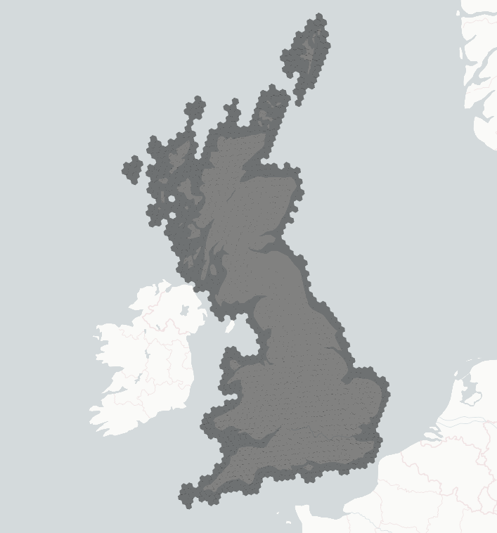
Map of Great Britain using H3 resolution 5
hexagons

Note: The generic geospatial logic for mapping latitude/longitude grids to H3 hexagons lives in the packages/geo package. This package (dynamical_data) focuses specifically on the ingestion, processing, and storage of time-varying NWP datasets like ECMWF. The H3 grid weights arrive as a Dagster asset from the geo package, so no precomputed static file is needed.

Data storage experiments

The storage format itself lives in delta_store.nwp (writer properties, sort order, precision); this section records the measurements behind it. Full before/after detail is in PR #271; earlier experiments (UInt8/Int16 affine quantisation, codec and sort-order sweeps) are in this file's git history. The same measure-before-you-optimise approach, and the storage numbers for the NWP table and the power_forecasts table side by side, are summarised in Performance and Scale. That page frames both tables' storage choices as an instance of design principle 12, measure; do not assume.

Current scheme: physical-unit Float32, every continuous variable rounded to a 13-bit significand (max relative error 2⁻¹³ ≈ 1.2×10⁻⁴ — measured ≤ 0.004 °C for temperature, ≤ 8 Pa for mean-sea-level (MSL) pressure), rows sorted init_time → ensemble_member → valid_time → h3_index, plain ZSTD level 3. init_time is when the weather model was run; valid_time is the moment being forecast.

Why round at all, when Dynamical.org already rounds? A significand is one bit wider than a mantissa, because the leading 1 is implicit, so 6–11 mantissa bits are 7–12 significand bits. Dynamical stores ECMWF ENS with 6–11 mantissa bits per variable (their binary_rounding.py). But trailing zeros do not survive arithmetic: our H3 aggregation is a weighted mean over grid points, and ECMWF publishes wind as an eastward component u and a northward component v, from which wind speed and direction are derived via sqrt/arctan2, so by the time values reach our writer their mantissas are full entropy again (measured: 100% of Dynamical-style rounded values have zeroed low bits; after a weighted mean, 0.07% do). Our 13-significand-bit rounding restores compressibility while being 1–6 bits finer than the upstream precision, so it discards almost nothing beyond what Dynamical already dropped.

How much space does Great-Britain-wide ECMWF ENS take? A lead time is one forecast step ahead of init_time. One daily run (1,671 H3 cells × 51 ensemble members × 85 lead times, up to ~7.24M rows) averages ~158 MB, so a year is ~58 GB. The full local development table — 899 daily runs (Apr 2024 → Sep 2026, ~6.5 billion rows) — is 142 GB.

Storage — the table below compares the writer configurations against each other, on nine real partitions spread across every season. The table's absolute figures are older than the NWP table on disk today. Every row was measured at parquet's default row-group size, against a partition set averaging 112.9 MB, where a partition now averages ~158 MB. The member-aligned row-group size that delta_store.nwp writes accounts for 8.6% of that difference, measured across the rewrite of all 899 partitions; the remaining 91.4% predates the member-aligned row-group size and is not accounted for here:

Config	avg MB/partition	extrapolated GB/yr
Previous: Int16 12-bit quantisation, ZSTD-14	115.3	42.1
Float32 + 13-bit significand, ZSTD-3	110.6	40.4
Adopted: same + member-early sort	112.9	41.2
Same + `BYTE_STREAM_SPLIT`	133.8	48.8

BYTE_STREAM_SPLIT makes this table worse (unlike power_forecasts, where it wins): significand rounding collapses NWP values into repeats that parquet's default dictionary+RLE encoding captures directly, and BYTE_STREAM_SPLIT scatters that repetition across four byte planes. Writer properties are data-dependent — measure per table.

Read path — the member-early sort puts each ensemble member's rows in one contiguous block, and delta_store.nwp sizes each parquet row group to hold exactly one member. Of the 51 members, member 0 is the unperturbed control run and the other 50 are perturbed. A single-member read (every training run reads just the control member) therefore matches one row group's min/max range and skips the other 50 row groups.

The read-path measurements below were taken on their own set of 29 consecutive daily partitions, not on the nine seasonal partitions the storage table above used. Measured against a valid_time-first sort of the same 29 daily partitions, reading nine H3 cells and the control member alone: 5.7× faster and 5.5× less peak memory (170 ms / 2,200 MB → 30 ms / 400 MB), for 3.7% more stored bytes (4.35 GB → 4.51 GB across the 29 partitions). Both tables were written freshly through write_nwp, differ only in the sort order, and use the member-aligned row-group size, so the comparison isolates the row order. Each figure is the warm-cache median of five timed repetitions.

The read decodes 1.96% of each partition censused — one row group in 51 — and that 1.96% holds for every member. A census of partitions from 2024, 2025, and 2026 found 51 row groups in each. Every row group spanned a single member, and the 51 together covered members 0 to 50, so no member decodes extra rows for sitting in the middle of the range. Under the valid_time-first sort the same read decodes 100%.

The timing and the peak-memory figures were both measured on local disk. On S3 a skipped row group also skips an HTTP range request over the internet, so both figures are a floor: the same read from S3 stands to gain more from row-group skipping.

# Two arms, one partition window, differing only in NWP_SORT_COLS; the second monkeypatches
# delta_store.nwp.NWP_SORT_COLS to ("init_time", "valid_time", "ensemble_member", "h3_index").
# Time each arm in its own process: ru_maxrss is a high-water mark that never falls, so two arms
# in one process report the larger figure twice.
frame = (
    Nwp.scan_delta(table)
    .filter(
        pl.col("init_time").is_between(window_start, window_end),
        pl.col("valid_time").is_between(window_start, window_end + timedelta(days=10)),
        pl.col("h3_index").is_in(cells),  # the 9 cells the 32 V1 series sit in
        pl.col("ensemble_member").is_in([0]),  # is_in, not ==, as load_engineering_inputs does
    )
    .collect(engine="streaming")
)

Per-variable keep_bits: considered and rejected (2026-07). Since Dynamical's upstream precision caps the real information at 7–12 significand bits per variable, budgets matched to upstream would compress better than the uniform 13. Measured on four seasonal partitions through the exact production write path (error columns = error added on top of today's stored values; wind speed's power impact is ~3× its relative error because the speed-to-power curve is roughly cubic):

Config	Size vs today	GB/yr	wind speed rel err	→ power (×3)	temp	MSL
Uniform 13 (today)	—	41.1	0	0	0	0
Upstream-matched (temp 8, wind 7, pressure 12, flux 8)	−19.4%	33.1	0.76%	2.3%	0.06 °C	16 Pa
Uniform 10	−15.6%	34.7	0.10%	0.29%	0.016 °C	64 Pa
Wind-protected (wind speed stays 13, rest squeezed)	−13.0%	35.7	0	0	0.06 °C	16 Pa

These figures share the Storage table's older ~41 GB/yr basis, so the percentage columns are comparable against each other but the absolute GB/yr sit below today's ~58 GB/yr.

The full squeeze adds ~2.3% power-equivalent wind error — not tolerable. The wind-safe ceiling is −13% ≈ 5.4 GB/yr, and the NWP table covers the whole of Great Britain, so it does not grow with the V2 scale-up to ~2,500 time series: a fixed ~5 GB/yr saving doesn't justify maintaining a dict of per-variable precision budgets. If disk ever becomes a real constraint, the wind-protected config is the one to reach for.

`dynamical_data.ecmwf_ens.download`

Opening and downloading one ECMWF ENS run from the Dynamical.org catalog.

Attributes

`ECMWF_ENS_INSTANTANEOUS_VARS = frozenset(_ECMWF_ENS_VARS_TO_DOWNLOAD) - Nwp.deaccumulated_var_names - Nwp.categorical_var_names` `module-attribute`

The downloaded variables describing conditions at one instant, under their download names.

None of these is ever legitimately null, anywhere in a run. That is why dynamical_data.ecmwf_ens.upstream_nulls.assess_upstream_grid_point_nulls counts them separately from the de-accumulated variables. It is also why the ecmwf_ens asset gates a check on that count being zero.

Derived from the download list rather than from Nwp's fields, because the two namespaces differ. We download wind_u_10m/wind_v_10m (and the 100 m pair), and dynamical_data.ecmwf_ens.convert_to_polars.convert_nwp_xarray_dataset_to_polars_dataframe derives wind_speed_*/wind_direction_* from them. A set taken from the contract would name four variables the downloaded dataset does not carry, and indexing it would raise KeyError.

Classes

`NwpRunNotYetAvailable`

Bases: Exception

Raised when nwp_init_time is not yet in the catalog.

Dynamical.org has not yet published that run.

Source code in packages/dynamical_data/src/dynamical_data/ecmwf_ens/download.py

class NwpRunNotYetAvailable(Exception):
    """Raised when ``nwp_init_time`` is not yet in the catalog.

    Dynamical.org has not yet published that run.
    """

Functions:

`open_ecmwf_ens_run(nwp_init_time, h3_grid)`

Lazily open the ECMWF ENS Icechunk store and slice it to the requested run and H3 grid.

No data is downloaded: the returned dataset is still backed by lazy Dask/Zarr arrays. Call download_ecmwf_ens_data to actually fetch the data.

Parameters:

Name	Type	Description	Default
`nwp_init_time`	`datetime`	The initialisation time to open. Must be timezone aware.	required
`h3_grid`	`DataFrame[H3GridWeights]`	The H3 grid to use for spatial bounds.	required

Returns:

Type	Description
`Dataset`	The catalog's dataset, sliced to the one `init_time` and to the latitude/longitude
`Dataset`	bounding box of `h3_grid`'s `nwp_lat`/`nwp_lon` columns, still lazy and holding the
`Dataset`	13 downloaded ECMWF ENS variables.

Source code in packages/dynamical_data/src/dynamical_data/ecmwf_ens/download.py

def open_ecmwf_ens_run(
    nwp_init_time: datetime,
    h3_grid: pt.DataFrame[H3GridWeights],
) -> xr.Dataset:
    """Lazily open the ECMWF ENS Icechunk store and slice it to the requested run and H3 grid.

    No data is downloaded: the returned dataset is still backed by lazy Dask/Zarr arrays.
    Call `download_ecmwf_ens_data` to actually fetch the data.

    Args:
        nwp_init_time: The initialisation time to open. Must be timezone aware.
        h3_grid: The H3 grid to use for spatial bounds.

    Returns:
        The catalog's dataset, sliced to the one `init_time` and to the latitude/longitude
        bounding box of `h3_grid`'s `nwp_lat`/`nwp_lon` columns, still lazy and holding the
        13 downloaded ECMWF ENS variables.
    """
    # Convention-sensitive to the *real* Dynamical.org catalog: this function bakes in assumptions
    # about its shape (longitude in [-180, 180], descending latitude, coordinate/dimension names).
    # The offline tests share those assumptions, so they cannot catch a mismatch with the live
    # catalog. After changing this function, run the network-gated test manually:
    #     uv run pytest --run-network -m network
    # See
    # <https://openclimatefix.github.io/nged-substation-forecast/architecture/testing/#network-gated-tests>.

    # Reusable-package input validation, not a reachable production state. The `ecmwf_ens` asset
    # always sources `h3_grid` from `h3_grid_weights`, which raises on an empty cell list before
    # writing anything. So the file that asset reads can never hold zero rows.
    if h3_grid.is_empty():
        raise ValueError("h3_grid is empty. Cannot download ECMWF data for an empty grid.")

    if nwp_init_time.utcoffset() is None:
        raise ValueError(f"nwp_init_time must be timezone aware. {nwp_init_time.tzinfo=}")

    # The xarray selection needs nwp_init_time timezone-naive, so nwp_init_time is converted to UTC
    # and then stripped of tzinfo here.
    utc_nwp_init_time = np.datetime64(nwp_init_time.astimezone(UTC).replace(tzinfo=None))

    ds = dynamical_catalog.open("ecmwf-ifs-ens-forecast-15-day-0-25-degree", chunks=None)

    ds = ds[list(_ECMWF_ENS_VARS_TO_DOWNLOAD)]

    if utc_nwp_init_time not in ds.init_time.values:
        raise NwpRunNotYetAvailable(f"{utc_nwp_init_time} is not in ds.init_time.values")

    # This check guards the Dynamical.org catalog itself, an external substrate we neither control
    # nor version-pin, so its shape can change under us between runs.
    if ds.longitude.size == 0 or ds.latitude.size == 0:
        raise ValueError("Dataset has empty longitude or latitude coordinates.")

    # Validate longitude range.
    # NOTE: Dynamical.org converts the longitude range to [-180, 180].
    if ds.longitude.min() < -180 or ds.longitude.max() > 180:
        raise ValueError("Dataset longitude must be in the range [-180, 180]")

    min_lat, max_lat, min_lon, max_lon = h3_grid.select(
        min_lat=pl.col("nwp_lat").min(),
        max_lat=pl.col("nwp_lat").max(),
        min_lon=pl.col("nwp_lon").min(),
        max_lon=pl.col("nwp_lon").max(),
    ).row(0)

    lat_slice = _calc_slice_for_lat_or_lng("latitude", ds, min_lat, max_lat)
    lon_slice = _calc_slice_for_lat_or_lng("longitude", ds, min_lon, max_lon)

    # NOTE: The slice below fails if the requested region crosses the anti-meridian. The GB
    # service area never does, so that case is not handled.
    ds_sliced = ds.sel(latitude=lat_slice, longitude=lon_slice, init_time=utc_nwp_init_time)

    # An empty spatial intersection here would otherwise surface much later as a confusing
    # KeyError during DataFrame conversion, so the intersection is checked and named explicitly now.
    if ds_sliced.longitude.size == 0 or ds_sliced.latitude.size == 0:
        raise ValueError("No spatial overlap found between H3 grid and NWP dataset.")

    return ds_sliced

`download_ecmwf_ens_data(ds_sliced)`

Download (compute) a lazily-opened, already-sliced ECMWF ENS dataset.

Parameters:

Name	Type	Description	Default
`ds_sliced`	`Dataset`	A lazy dataset as returned by `open_ecmwf_ens_run`.	required

Returns:

Type	Description
`Dataset`	The same variables and coordinates as `ds_sliced`. Each variable is now backed by an
`Dataset`	in-memory `xr.DataArray` rather than a lazy Dask/Zarr array. Up to four variables are
`Dataset`	downloaded concurrently.

Source code in packages/dynamical_data/src/dynamical_data/ecmwf_ens/download.py

def download_ecmwf_ens_data(ds_sliced: xr.Dataset) -> xr.Dataset:
    """Download (compute) a lazily-opened, already-sliced ECMWF ENS dataset.

    Args:
        ds_sliced: A lazy dataset as returned by `open_ecmwf_ens_run`.

    Returns:
        The same variables and coordinates as `ds_sliced`. Each variable is now backed by an
        in-memory `xr.DataArray` rather than a lazy Dask/Zarr array. Up to four variables are
        downloaded concurrently.
    """

    def download_array(var_name: str) -> dict[str, xr.DataArray]:
        return {var_name: ds_sliced[var_name].compute()}

    # The download is I/O bound (S3 network requests). We use a ThreadPoolExecutor to parallelise
    # network latency across multiple variables. A ProcessPoolExecutor would be less efficient here
    # due to the high serialisation overhead of Xarray objects between processes.
    #
    # max_workers is capped rather than left at the default (one thread per variable, i.e. 13).
    # Investigation of issue #276 found that 13 concurrent chunked-zarr fetches self-contend badly
    # (S3 rate limiting or connection-pool starvation). Most variables finish in 5-20s, but a few
    # straggle for minutes, which makes the whole download 600s+. Capping at 4 removed the
    # stragglers entirely and cut a real download from 645s to 22.5s.
    #
    # 4 is the cap *per partition*, not per machine. `ecmwf_ens` runs up to its `ECMWF` pool limit
    # of partitions at once (4, set in `dagster.yaml`), so the fetches in flight against
    # Dynamical.org are the product of the two. Lower this cap before raising that limit.
    #
    # The slowdown is a recent regression, not a pre-existing property of the download. Dagster's
    # run history shows per-partition downloads holding a steady ~48-54s right up to 2026-06-30
    # 12:26 UTC. Every run afterwards (2026-07-01 onwards) took 3-12 min. That boundary
    # lines up exactly with an `icechunk` 2.0.6 -> 2.1.0 bump in the same `uv.lock` update
    # (commit b46d145, 2026-06-30 12:26:50 UTC). The leading theory is a change in icechunk's
    # underlying S3 client (connection pooling/concurrency handling) between those two versions.
    # That theory has not been confirmed by pinning back to 2.0.6 and re-testing.
    data_arrays: dict[str, xr.DataArray] = {}
    with concurrent.futures.ThreadPoolExecutor(max_workers=4) as executor:
        futures = [executor.submit(download_array, str(name)) for name in ds_sliced.data_vars]
        for future in concurrent.futures.as_completed(futures):
            data_arrays.update(future.result())

    return xr.Dataset(data_arrays)

`dynamical_data.ecmwf_ens.convert_to_polars`

Converting a downloaded ECMWF ENS xarray dataset into the Nwp Polars contract.

The regular lat/lon grid is aggregated onto H3 cells on the way.

Attributes

Classes

Functions:

`convert_nwp_xarray_dataset_to_polars_dataframe(ds, h3_grid)`

Convert one downloaded ECMWF ENS run into the validated Nwp frame.

Loops over every (lead_time, ensemble_member) pair in ds. For each pair, aggregates that chunk's grid points onto h3_grid's H3 cells and derives wind speed and direction from the downloaded u/v components. Returns the concatenated result, validated against the Nwp contract.

Guarantees, per cell:

A numeric variable is the area-weighted mean of the points that supplied a value. The numerator is sum(v * p), where the proportion weights p sum to 1 over the whole cell by construction (see geo.h3.compute_h3_grid_weights). The denominator is the contributing weight rather than that 1.0, so a missing point takes only its own share out of the cell instead of biasing the cell low.
A categorical variable is the category covering most of the cell's area, with an exact tie resolved to the lowest category code. Points that supplied no category are excluded from the ranking rather than competing in it.
Either kind yields null, never 0.0 or a spurious category, when no point contributed.

Each variable is renormalised over its own denominator, which is what keeps one variable's corruption from nulling the others. The cost a caller must know about: two variables in one cell can then be averaged over different sub-areas of the hexagon. So if wind_u_* and wind_v_* ever have different null footprints, the wind vector derived by _calc_wind_speed and _calc_wind_direction mixes two sub-areas. Upstream corruption has always been co-located across variables, so that is theoretical today.

Parameters:

Name	Type	Description	Default
`ds`	`Dataset`	One downloaded ECMWF ENS run, as returned by `dynamical_data.ecmwf_ens.download.download_ecmwf_ens_data` — dimensions `(lead_time, ensemble_member, latitude, longitude)`, with `init_time` a scalar coordinate, and carrying the 13 downloaded ECMWF ENS variables.	required
`h3_grid`	`DataFrame[H3GridWeights]`	The H3 grid weights to aggregate onto. One row per (H3 cell, NWP grid point) pair whose cell and grid point overlap. `proportion` is the fraction of that cell's area the point covers.	required

Returns:

Type	Description
`DataFrame[Nwp]`	One row per `(init_time, valid_time, ensemble_member, h3_index)`, validated against `Nwp`.
`DataFrame[Nwp]`	The wind components are dropped in favour of the derived speed and direction. Every other
`DataFrame[Nwp]`	downloaded variable is carried through under its `Nwp` field name.

Source code in packages/dynamical_data/src/dynamical_data/ecmwf_ens/convert_to_polars.py

def convert_nwp_xarray_dataset_to_polars_dataframe(
    ds: xr.Dataset,
    h3_grid: pt.DataFrame[H3GridWeights],
) -> pt.DataFrame[Nwp]:
    """Convert one downloaded ECMWF ENS run into the validated `Nwp` frame.

    Loops over every `(lead_time, ensemble_member)` pair in `ds`. For each pair, aggregates that
    chunk's grid points onto `h3_grid`'s H3 cells and derives wind speed and direction from the
    downloaded u/v components. Returns the concatenated result, validated against the `Nwp`
    contract.

    Guarantees, per cell:

    - A **numeric** variable is the area-weighted mean of the points that supplied a value. The
      numerator is `sum(v * p)`, where the `proportion` weights `p` sum to 1 over the whole cell by
      construction (see `geo.h3.compute_h3_grid_weights`). The denominator is the *contributing*
      weight rather than that 1.0, so a missing point takes only its own share out of the cell
      instead of biasing the cell low.
    - A **categorical** variable is the category covering most of the cell's area, with an exact
      tie resolved to the lowest category code. Points that supplied no category are excluded from
      the ranking rather than competing in it.
    - Either kind yields **null**, never `0.0` or a spurious category, when *no* point contributed.

    Each variable is renormalised over its *own* denominator, which is what keeps one variable's
    corruption from nulling the others. The cost a caller must know about: two variables in one
    cell can then be averaged over different sub-areas of the hexagon. So if `wind_u_*` and
    `wind_v_*` ever have different null footprints, the wind vector derived by `_calc_wind_speed`
    and `_calc_wind_direction` mixes two sub-areas. Upstream corruption has always been co-located
    across variables, so that is theoretical today.

    Args:
        ds: One downloaded ECMWF ENS run, as returned by
            `dynamical_data.ecmwf_ens.download.download_ecmwf_ens_data` — dimensions
            `(lead_time, ensemble_member, latitude, longitude)`, with `init_time` a scalar
            coordinate, and carrying the 13 downloaded ECMWF ENS variables.
        h3_grid: The H3 grid weights to aggregate onto. One row per (H3 cell, NWP grid point) pair
            whose cell and grid point overlap. `proportion` is the fraction of that cell's area the
            point covers.

    Returns:
        One row per `(init_time, valid_time, ensemble_member, h3_index)`, validated against `Nwp`.
        The wind components are dropped in favour of the derived speed and direction. Every other
        downloaded variable is carried through under its `Nwp` field name.
    """
    # Convention-sensitive to real ECMWF ENS data. The dimension and coordinate order feeds the
    # ravel below and the value-join that follows it, and the physical units feed Nwp.validate. The
    # offline tests share those assumptions, so after changing this function run the network-gated
    # test manually:
    #     uv run pytest --run-network -m network
    # See
    # <https://openclimatefix.github.io/nged-substation-forecast/architecture/testing/#network-gated-tests>.

    # Precompute latitude and longitude grids
    lat_grid, lon_grid = np.meshgrid(
        ds.latitude.values.astype(np.float32),
        ds.longitude.values.astype(np.float32),
        indexing="ij",
    )
    lat_grid_raveled = lat_grid.ravel()
    lon_grid_raveled = lon_grid.ravel()

    # Iterate over lead_time and ensemble_member to process in chunks.
    dfs: list[pl.DataFrame] = []
    for lead_time in ds.lead_time.values:
        for ensemble_member in ds.ensemble_member.values:
            ds_chunk = ds.sel(lead_time=lead_time, ensemble_member=ensemble_member)
            df = _process_chunk_for_1_lead_time_and_1_ens_member(
                ds_chunk,
                h3_grid,
                lat_grid=lat_grid_raveled,
                lon_grid=lon_grid_raveled,
            ).with_columns(
                ensemble_member=pl.lit(ensemble_member).cast(pl.Int8),
                valid_time=pl.lit(ds_chunk["valid_time"].values).cast(UTC_DATETIME_DTYPE),
            )
            dfs.append(df)

    df = (
        pl.concat(dfs)
        .with_columns(
            nwp_model_id=pl.lit(NwpModelId.ECMWF_ENS_0_25_degree.name).cast(pl.String),
            init_time=pl.lit(ds["init_time"].values).cast(UTC_DATETIME_DTYPE),
            # h3_grid.h3_index (H3GridWeights, joined in above) is UInt64. That contract is
            # Parquet-backed, so it never had Delta's no-unsigned-integer constraint. Nwp.h3_index
            # is Int64, so the cast belongs here rather than at H3GridWeights's boundary. The
            # narrowing loses nothing at any resolution: H3 reserves bit 63 of every index as zero,
            # so no H3 value reaches the bit a signed Int64 gives up. See Nwp.h3_index in
            # contracts.weather_schemas for the full argument.
            h3_index=pl.col("h3_index").cast(pl.Int64),
            # Wind speed and direction are computed here, after the H3 aggregation above, and that
            # order matters. wind_u_*/wind_v_* are aggregated as ordinary numeric variables first.
            # Speed and direction are then derived from the already-aggregated components. Averaging
            # *direction* over grid points instead would average bearings numerically, and two
            # points either side of North would come out as due South. A naive time resample of a
            # direction column hits that same 0/360 wrap defect. See
            # <https://openclimatefix.github.io/nged-substation-forecast/architecture/nwp-variable-conventions/#wind-is-stored-as-speed-and-direction-and-why>.
            wind_speed_10m=_calc_wind_speed(height="10m"),
            wind_speed_100m=_calc_wind_speed(height="100m"),
            wind_direction_10m=_calc_wind_direction(height="10m"),
            wind_direction_100m=_calc_wind_direction(height="100m"),
        )
        .drop(cs.matches("^wind_u_.*") | cs.matches("^wind_v_.*"))
    )

    # No sort here: physical row order is delta_store.nwp's job (the single source of truth for
    # on-disk layout), and validation is order-independent.
    return Nwp.validate(df)

`dynamical_data.ecmwf_ens.upstream_nulls`

Measuring upstream corruption on the raw NWP grid, before the H3 aggregation sees it.

The H3 aggregation renormalises each cell over the grid points that supplied a value, so a corrupt grid point costs only its own share of its cell. That renormalisation is what makes the stored cells robust. That renormalisation is also why counting null cells is a poor proxy for how corrupt the feed was. This module counts the nulls where they arrive, before that renormalisation absorbs most of them. The aggregation mechanics are documented, along with the measurements behind the claim that a corrupt grid point takes only its own share out of its cell, at https://openclimatefix.github.io/nged-substation-forecast/architecture/ecmwf-ens-known-issues/#spatial-aggregation-is-where-a-grid-points-null-is-resolved.

Classes

`UpstreamNullRate` `dataclass`

How much of one ingested NWP run arrived null on the raw grid.

This is the provider channel: the number to quote to Dynamical.org when asking whether their feed is degrading. It counts grid points on the 0.25° lat/lon box we downloaded, before any H3 aggregation.

Read it alongside contracts.weather_schemas.NwpQualityReport, never instead of that report. NwpQualityReport counts null H3 cells and answers the different question of how much the power-forecasting model lost. The two are not comparable as rates: different units over different populations.

See https://openclimatefix.github.io/nged-substation-forecast/architecture/ecmwf-ens-known-issues/.

Source code in packages/dynamical_data/src/dynamical_data/ecmwf_ens/upstream_nulls.py

@dataclass(frozen=True)
class UpstreamNullRate:
    """How much of one ingested NWP run arrived null on the **raw grid**.

    This is the provider channel: the number to quote to Dynamical.org when asking whether their
    feed is degrading. It counts grid points on the 0.25° lat/lon box we downloaded, before any
    H3 aggregation.

    Read it alongside `contracts.weather_schemas.NwpQualityReport`, never instead of that report.
    `NwpQualityReport` counts null H3 *cells* and answers the different question of how much the
    power-forecasting model lost. The two are not comparable as rates: different units over
    different populations.

    See
    <https://openclimatefix.github.io/nged-substation-forecast/architecture/ecmwf-ens-known-issues/>.
    """

    per_variable: pl.DataFrame
    """One row per counted variable, with its ``n_null``, ``n_affected_slices`` and ``n_total``
    grid-point counts, sorted by variable name. Every scalar below is derived from it, so a
    breakdown and a total cannot disagree."""

    @property
    def n_null_nwp_grid_points(self) -> int:
        """Null grid points in the counted variables and steps."""
        return int(self.per_variable["n_null"].sum())

    @property
    def n_total_nwp_grid_points(self) -> int:
        """The denominator: counted variables × ensemble members × counted steps × grid points."""
        return int(self.per_variable["n_total"].sum())

    @property
    def n_affected_nwp_slices(self) -> int:
        """``(variable, ensemble_member, lead_time)`` slices carrying at least one null grid point.

        Separates "one bad slice" from "a hundred" at the same overall rate, which the fraction
        alone cannot.
        """
        return int(self.per_variable["n_affected_slices"].sum())

    @property
    def affected_nwp_variables(self) -> tuple[str, ...]:
        """The counted variables carrying at least one null grid point.

        In ``per_variable``'s row order, which is sorted by variable name because
        `assess_upstream_grid_point_nulls` builds it that way. ``filter`` preserves row order
        rather than imposing a row order.
        """
        return tuple(self.per_variable.filter(pl.col("n_null") > 0)["variable"])

    @property
    def null_nwp_grid_point_fraction(self) -> float:
        """Null grid points as a fraction of those counted; ``0.0`` when none were counted.

        A run with no step left to count has nothing to measure, and a warning path must not
        raise ([rule
        7](https://openclimatefix.github.io/nged-substation-forecast/design-philosophy/inherent-stability/#the-rules)).
        """
        if self.n_total_nwp_grid_points == 0:
            return 0.0
        return self.n_null_nwp_grid_points / self.n_total_nwp_grid_points

    @property
    def is_healthy(self) -> bool:
        """True when no counted grid point arrived null."""
        return self.n_null_nwp_grid_points == 0

Attributes

`per_variable` `instance-attribute`

One row per counted variable, with its n_null, n_affected_slices and n_total grid-point counts, sorted by variable name. Every scalar below is derived from it, so a breakdown and a total cannot disagree.

`n_null_nwp_grid_points` `property`

Null grid points in the counted variables and steps.

`n_total_nwp_grid_points` `property`

The denominator: counted variables × ensemble members × counted steps × grid points.

`n_affected_nwp_slices` `property`

(variable, ensemble_member, lead_time) slices carrying at least one null grid point.

Separates "one bad slice" from "a hundred" at the same overall rate, which the fraction alone cannot.

`affected_nwp_variables` `property`

The counted variables carrying at least one null grid point.

In per_variable's row order, which is sorted by variable name because assess_upstream_grid_point_nulls builds it that way. filter preserves row order rather than imposing a row order.

`null_nwp_grid_point_fraction` `property`

Null grid points as a fraction of those counted; 0.0 when none were counted.

A run with no step left to count has nothing to measure, and a warning path must not raise (rule 7).

`is_healthy` `property`

True when no counted grid point arrived null.

Methods:

`init(per_variable)`

Functions:

`assess_upstream_grid_point_nulls(ds, variables, exclude_lead_0)`

Count nulls on the raw NWP grid of one downloaded run.

Pure and Dagster-free (unit-testable in isolation). The ecmwf_ens asset calls it twice, once per null population, and publishes each result on its own WARN check.

Parameters:

Name	Type	Description	Default
`ds`	`Dataset`	One downloaded ECMWF ENS run, as returned by `dynamical_data.ecmwf_ens.download.download_ecmwf_ens_data` — dimensions `(lead_time, ensemble_member, latitude, longitude)`, with `init_time` already reduced to a scalar coordinate.	required
`variables`	`Collection[str]`	The variables to count over, named as `ds` names them rather than as the `Nwp` contract does — the two differ on wind, so `dynamical_data.ecmwf_ens.download.ECMWF_ENS_INSTANTANEOUS_VARS` exists to be passed here. Their nulls must share one meaning, because it measures nothing to pool a rate over variables with opposite null semantics. The asset therefore makes two separate calls. One call passes the de-accumulated variables, which Dynamical.org differences from ECMWF's running totals into rates (`W m-2` for the radiation fluxes, `kg m-2 s-1` for precipitation), so their nulls are known upstream corruption. The other call passes the instantaneous variables, whose nulls are anomalous.	required
`exclude_lead_0`	`bool`	Skip the lead-0 step. True for the de-accumulated variables, which are null there by design, so counting it would report every healthy run as corrupt. False for the instantaneous ones, where lead-0 is an ordinary step and a null in it means what a null in any other step means.	required

Returns:

Type	Description
`UpstreamNullRate`	An `UpstreamNullRate` whose `per_variable` frame holds one row per counted variable, sorted
`UpstreamNullRate`	by variable name. Each row gives that variable's null grid-point count (`n_null`), the count
`UpstreamNullRate`	of (ensemble_member, lead_time) slices holding at least one null (`n_affected_slices`), and
`UpstreamNullRate`	the total number of grid points counted (`n_total`).

Source code in packages/dynamical_data/src/dynamical_data/ecmwf_ens/upstream_nulls.py

def assess_upstream_grid_point_nulls(
    ds: xr.Dataset, variables: Collection[str], exclude_lead_0: bool
) -> UpstreamNullRate:
    """Count nulls on the raw NWP grid of one downloaded run.

    Pure and Dagster-free (unit-testable in isolation). The ``ecmwf_ens`` asset calls it twice, once
    per null population, and publishes each result on its own WARN check.

    Args:
        ds: One downloaded ECMWF ENS run, as returned by
            `dynamical_data.ecmwf_ens.download.download_ecmwf_ens_data` — dimensions
            ``(lead_time, ensemble_member, latitude, longitude)``, with ``init_time`` already
            reduced to a scalar coordinate.
        variables: The variables to count over, named as ``ds`` names them rather than as the
            ``Nwp`` contract does — the two differ on wind, so
            `dynamical_data.ecmwf_ens.download.ECMWF_ENS_INSTANTANEOUS_VARS` exists to be
            passed here. Their nulls must share one meaning, because it measures nothing to pool a
            rate over variables with opposite null semantics. The asset therefore makes two separate
            calls. One call passes the de-accumulated variables, which Dynamical.org differences
            from ECMWF's running totals into rates (``W m-2`` for the radiation fluxes, ``kg m-2
            s-1`` for precipitation), so their nulls are known upstream corruption. The other call
            passes the instantaneous variables, whose nulls are anomalous.
        exclude_lead_0: Skip the lead-0 step. True for the de-accumulated variables, which are null
            there by design, so counting it would report every healthy run as corrupt. False for
            the instantaneous ones, where lead-0 is an ordinary step and a null in it means what a
            null in any other step means.

    Returns:
        An `UpstreamNullRate` whose `per_variable` frame holds one row per counted variable, sorted
        by variable name. Each row gives that variable's null grid-point count (`n_null`), the count
        of (ensemble_member, lead_time) slices holding at least one null (`n_affected_slices`), and
        the total number of grid points counted (`n_total`).
    """
    # Selected per variable rather than once on `ds`. This code runs inside `ecmwf_ens` while the
    # whole downloaded run is still held in memory. Slicing the whole dataset would copy all 13
    # downloaded variables to read either the three de-accumulated variables or the nine
    # instantaneous variables, depending on the call. The 13th is
    # categorical_precipitation_type_surface, which neither call counts.
    beyond_lead_0 = ds.lead_time > _LEAD_0
    rows = []
    for name in sorted(variables):
        values = ds[name].isel(lead_time=beyond_lead_0) if exclude_lead_0 else ds[name]
        nulls_per_slice = values.isnull().sum(dim=["latitude", "longitude"])
        rows.append(
            {
                "variable": name,
                "n_null": int(nulls_per_slice.sum()),
                "n_affected_slices": int((nulls_per_slice > 0).sum()),
                "n_total": values.size,
            }
        )
    return UpstreamNullRate(per_variable=pl.DataFrame(rows, schema=_PER_VARIABLE_SCHEMA))

Dynamical Data API

Dynamical Data Package

Data storage experiments

dynamical_data.ecmwf_ens.download

Attributes

ECMWF_ENS_INSTANTANEOUS_VARS = frozenset(_ECMWF_ENS_VARS_TO_DOWNLOAD) - Nwp.deaccumulated_var_names - Nwp.categorical_var_names module-attribute

Classes

NwpRunNotYetAvailable

Functions:

open_ecmwf_ens_run(nwp_init_time, h3_grid)

download_ecmwf_ens_data(ds_sliced)

dynamical_data.ecmwf_ens.convert_to_polars

Attributes

Classes

Functions:

convert_nwp_xarray_dataset_to_polars_dataframe(ds, h3_grid)

dynamical_data.ecmwf_ens.upstream_nulls

Classes

UpstreamNullRate dataclass

Attributes

per_variable instance-attribute

n_null_nwp_grid_points property

n_total_nwp_grid_points property

n_affected_nwp_slices property

affected_nwp_variables property

null_nwp_grid_point_fraction property

is_healthy property

Methods:

__init__(per_variable)

Functions:

assess_upstream_grid_point_nulls(ds, variables, exclude_lead_0)

`dynamical_data.ecmwf_ens.download`

`ECMWF_ENS_INSTANTANEOUS_VARS = frozenset(_ECMWF_ENS_VARS_TO_DOWNLOAD) - Nwp.deaccumulated_var_names - Nwp.categorical_var_names` `module-attribute`

`NwpRunNotYetAvailable`

`open_ecmwf_ens_run(nwp_init_time, h3_grid)`

`download_ecmwf_ens_data(ds_sliced)`

`dynamical_data.ecmwf_ens.convert_to_polars`

`convert_nwp_xarray_dataset_to_polars_dataframe(ds, h3_grid)`

`dynamical_data.ecmwf_ens.upstream_nulls`

`UpstreamNullRate` `dataclass`

`per_variable` `instance-attribute`

`n_null_nwp_grid_points` `property`

`n_total_nwp_grid_points` `property`

`n_affected_nwp_slices` `property`

`affected_nwp_variables` `property`

`null_nwp_grid_point_fraction` `property`

`is_healthy` `property`

`init(per_variable)`

`assess_upstream_grid_point_nulls(ds, variables, exclude_lead_0)`