Inherent Stability

We never stop forecasting power. When an input goes missing or stale, the forecast degrades gracefully instead of stopping: it becomes less certain, and it says so, through wider uncertainty bands. Wherever possible, that stability should be an inherent property of the system's design, rather than something bolted on afterwards by post-processing and if-then-else branches in the production service.

This page argues in full the first and largest of the project's design principles: how Flexpectation behaves when its inputs degrade. It is the how behind H1 — the hypothesis that the service mostly runs itself. The rules below are the fine-grained form of the never-stop, complexity-offline and strict-contracts principles in that list.

The model does the work, not a fallback path. A central mechanism behind everything below is that the ML model itself is built to keep producing a sensible forecast when some of its inputs are missing — rather than a chain of fallbacks wrapped around a model that assumes complete data. That is already partly true: the gradient-boosted trees we run today route missing features instead of requiring them to be filled in, so a forecast still comes out when a feature drops away. But the model has not yet been trained against realistic outages, which is what turns "it still produces a number" into "it still produces a number worth trusting". Much of what follows — the degradation ladder, the widening bands, the failure-scenario suite — exists to make that one design choice work; the mechanics are in Default directions, and their limit and Missingness in learned models.

Scope. The principle and the mechanisms that already exist are described here. Mechanisms that are designed but not yet built are linked, not copied — they live in docs/roadmap/ until they ship, and duplicating them here would make this page a roadmap mirror that rots. Sections carry the usual status markers: ✅ implemented, 🚧 designed but not built.

What is "inherent stability"?

If you have ever built and ridden a simple "soap box" cart, you will know that the steering is worryingly unstable: you have to fight it constantly to keep the cart going straight. Let go of the steering ropes and the wheels whip hard left or hard right, probably ending in a crash. The machine is trying to hurt you! It is inherently unstable, and it requires constant, active control to keep it safe.

A soap box cart, 1950. The whole steering mechanism is a front axle that pivots under the plank, pulled left or right by the length of string in the rider's hand. That pivot is vertical, so nothing returns the axle to centre. Photo from the Nationaal Archief, resized, used under CC BY-SA 3.0.

A proper car's steering is the stark contrast. Its front wheels do not pivot about a vertical axis, as the cart's do. Each one turns about a kingpin — the pin at the outer end of the axle, which carries the steering knuckle the wheel is bolted to — and that pin is deliberately tilted, both backwards (the castor angle) and inwards (kingpin inclination). The backward tilt is the important one here: it makes the steering axis meet the road slightly ahead of the point where the tyre actually touches it, which leaves each wheel trailing behind its own pivot, exactly like the castor on an office chair or the front wheel of a bicycle.

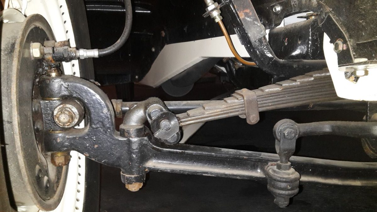
The same job done properly: a car's front axle, with the kingpin and steering knuckle at the wheel end and the track rod running across to the other wheel. The tilt built into that pin is what makes the steering self-centring. Photo by Dr.-Ing. S. Wetzel of an exhibit in the August Horch Museum, Zwickau, via Wikimedia Commons, resized, copyrighted free use.

The effect has a name: self-aligning torque. Any deviation from straight-ahead generates a force that pulls the wheel back towards the centre, and the vehicle-level property it produces is called directional stability. Let go of the steering wheel and it returns to centre on its own. No sensor measures that error and no controller corrects it: the geometry is chosen so that the physics does the work. The machine is trying to keep you safe, not through lots of active control, but by its very shape.

That is what we want from the forecasting service. Wherever we can manage it, sensible behaviour under disturbance should fall out of how the system is built, rather than being watched for and corrected by machinery bolted on around it.

NGED's incumbent forecast is the floor

Even in the worst case, when we have no fresh data, we hope to still be able to provide a better power forecast that NGED's incumbent forecast, with appropriate confidence bands. This is what allows us to claim that we should always be able to produce a power forecast, even when "blind".

NGED's incumbent forecast assembles 13 historical analogues at the same time-of-day on the same weekday — 6 from the last 6 weeks, 7 from 49–55 weeks back — and reads them as an ensemble. No weather, no ML, no holiday alignment, no load-growth scaling.

Two of its properties set our floor. It consumes no NWP, so an NWP outage does not degrade it at all — which makes an NWP outage the hard test for us. And it survives a power-data outage, because the 49–55-week-old analogues are indifferent to recent staleness. The incumbent already embodies this philosophy, which is why it is the right thing to measure ourselves against, and it gives a far better failure criterion than any arbitrary staleness threshold:

We should only fail when we can no longer beat the incumbent.

The consequence, once verified, is the strongest claim on this page:

At our worst we degrade to roughly the incumbent. At our best we beat it substantially. There is no state in which NGED is worse off than they are today.

That is currently an intention, not a measured fact. Making it measurable needs the nged_incumbent baseline (Metrics & Leaderboard → The headline baseline, #147) and a failure-scenario suite to score against it. Until both exist, treat the claim as the thing we are trying to earn.

The degradation ladder

Rung	Available inputs	Expected behaviour
0	Everything fresh	Best skill; narrowest bands
1	One or two daily NWP runs missed	Slightly worse; bands widen slightly
2	No NWP for days or weeks	Weather-blind: lags, calendar, per-series structure. Should still beat the incumbent
3	No NWP and no recent power	Calendar + climatology + year-old history. Converges toward being the incumbent
4	Nothing at all	Physical envelope (clear-sky) + climatology. Very wide bands, still bounded and still true

Rung 4 matters because it demonstrates that there is no input state in which we have nothing true to say: clear-sky irradiance needs only latitude, longitude and time.

Rungs are counted in missed NWP runs, never in hours of staleness — see Three audiences, three channels for why raw age is not a health signal.

Three related words are used deliberately across these pages. A regime is one cell of the input-availability grid — NWP × telemetry × metadata, ten to twenty realistic combinations. A scenario is a regime's named, versioned realisation in the failure-scenario suite. A rung of this ladder is a severity band of regimes.

Failure modes

What breaks, what the system does about it, and whether anyone is alerted. "Today" describes the code as it stands; "intended" describes where this principle takes it.

Failure	Today	Intended	Human alerted?
One or two daily NWP runs missed	live_forecasts selects the freshest run present as of the forecast time, so an older run is used through the normal path; live_forecasts_are_healthy warns with the count of missed runs	Unchanged	No
NWP stale but still covering the horizon	Forecast produced from an increasingly ancient run; nwp_init_time is on every row and live_forecasts_are_healthy warns with the missed-run count, but the forecast itself looks as confident as a fresh one	Bands widen with the regime; STALE NWP warning row 🚧	No
A slot produces no rows, or unusable ones, while the asset still succeeds	live_forecasts_are_healthy warns, naming the row count, the invalid rows and any trained series that went missing	Unchanged	No
NWP absent, or too old to cover the horizon	Hard failure — the asset raises and NGED gets nothing (tracked to change in #446)	Weather-blind forecast, wide bands, warning row 🚧	No
Telemetry stalled for one series	Forecast still produced from the model's other features; power_data_is_fresh warns and names the late series	Unchanged, plus regime-appropriate band widening 🚧	No
A meter reporting detectably wrong values	Partly detected at ingest; see Missing versus wrong	Treated as missing, which routes it into the always-output path 🚧	No
A whole ECMWF slice corrupt	Landed; nwp_has_no_unexpected_nulls warns, naming the slice	Unchanged	No
A whole ECMWF weather variable absent	Nwp.validate rejects it; ecmwf_ens turns each rejection into a retry for up to 4h, and once those are exhausted it manifests downstream as a missed run	Unchanged	No
The promoted model is empty or unloadable	Hard failure — the asset raises	Unchanged: this is a promotion bug, not a data outage	Yes, next business day
The service is not running at all	Sentry missed-check-in alarm fires from outside the deployment	Unchanged	Yes, next business day
Any of the above during model R&D	Fails fast	Unchanged — see R&D fails the other way	n/a

Nothing here is a 2am page. The uptime posture that makes that acceptable is argued in Requirements → Uptime: lenient by design.

The rules

These are the imperative form of everything above: the checklist to follow when in doubt while changing production code. It is deliberately self-contained, so some of them restate a design principle rather than adding anything new. Those are marked below — if you change one, change its matching principle too. The rest are specific to degradation and appear nowhere else.

1. In production, never raise because an input is absent or stale. Degrade, widen the bands, and record the degradation on the row. Reserve raising for states that are our own bug — an empty promoted model, a contract violation — not for the outside world misbehaving. (The never-stop principle, in imperative form.)
2. Be liberal about missing inputs and strict about malformed ones. Absent data routes into the always-output path; malformed data is rejected at the contract boundary. These are opposite postures and both are deliberate. (The strict-contracts principle, in imperative form.)
3. Treat detectably-wrong input as missing, not as data — see Missing versus wrong.
4. Signal degradation in-band first. The uncertainty band is the only number the consumer is certain to read. Side channels — warning tables, checks, Sentry — supplement it; they never substitute for it.
5. Measure degradation in missed runs and absent inputs, never in raw hours of age. Healthy NWP is between 12 and 30 hours old depending on the slot, so an absolute age threshold is either a daily false alarm or a magic number silently coupled to the ingest schedule — and either way it cannot say how many runs are missing.
6. Asset checks warn; they do not block. AssetCheckSeverity.WARN with blocking=False is the house pattern, and there is deliberately no ERROR-severity check anywhere in the repo.
7. Never let the warning path be able to fail the thing it is warning about. A bug in a warning function that raises would convert fail-open into fail-closed at exactly the wrong moment, which is why report_power_freshness never raises and why both asset checks (power_data_is_fresh, live_forecasts_are_healthy) run their whole body under a catch-all. Non-blocking is not enough on its own: Dagster fails a run whose check step errors, whatever its blocking setting, and the scheduled jobs carry a Sentry failure hook — so an unguarded warning path both fails the run and pages.
8. When a capability could live in the training loop or in the production service, put it in the training loop. See Where complexity should live. (The complexity-offline principle, in imperative form.)
9. Fail in the direction where being wrong is cheapest to recover from. In production that is forward; in model R&D it is backward. See R&D fails the other way.
10. Damp the corrections. Bounded retries with backoff, rate limits on retraining and hysteresis on model promotion (the latter two designed but not built 🚧) are as much a part of this principle as the degradation ladder is.
11. Never make one production job's run status a precondition for another's. Couple them through data at rest: read whatever is on disk, note which run it came from, and carry on. A dependency in the lineage graph is fine and useful — it is what lets a developer ask for an asset and its upstreams together on a laptop — but it must never become a runtime gate. A gate turns one failed upstream run into a missing forecast, and a missing forecast is not on the ladder at all: not even rung 4, where the service still emits a very wide but true forecast. (The coupling-through-data-at-rest principle, in imperative form.)

Where complexity should live

When a capability can be built into the training loop or into the production service, build it into the training loop.

The service runs unattended at 06:00 on the day the inputs are strangest. Training runs in front of a human who can read the traceback and re-run it. Complexity in the two places therefore carries very different risk, and the same reasoning that puts fail-fast in R&D and fail-operational in production says the same thing about where code should sit: keep the serving path as close to "load a model, call predict" as we can.

This is descriptive as much as aspirational. promoted_model already copies the champion to local disk so that inference makes no MLflow call. Regime-conditional interval calibration has the same shape: computed offline, and production does a table lookup.

Two qualifiers keep it honest.

• It is a tie-break, not an override. A single model spanning every degradation regime may spend capacity on regimes that occur one day in a hundred. Where skill is comparable, prefer the simpler service; where the gap is measured and real, skill wins.

• It relocates the branch rather than removing it. A fallback cascade's if is reviewable and directly testable; a model that "handles anything" holds the same branch internally, as a learned default direction, and that can only be measured. The principle is therefore safe to apply only once a failure-scenario suite exists to measure it.

It does not license unbounded training complexity, either: a training harness nobody can run is also a production risk, because H2 and H3 depend on retraining staying cheap and promotion staying one command.

Mechanisms

Missing versus wrong

"Always output" is not "always trust".

• Absent or stale input → always produce a forecast. Degrade, widen, declare.
• Detectably wrong input → do not consume it. Treat it as missing, which routes it back into the always-output path.

A stuck meter reporting 2.1 MW for 52 hours is not missing data; it is actively misleading, and a lag-feature model will propagate it happily. The incumbent has the identical vulnerability. Data Quality documents both classes empirically — false zeros, stuck values and genuinely missing data as separate phenomena — and is the evidence base for this distinction.

Default directions, and their limit

XGBoost uses sparsity-aware split finding. At every split it learns not just a threshold but a default direction for rows where that feature is missing: it tries sending all missing rows left, then right, and keeps whichever gives better gain. Missingness is routed, not imputed. This is why a leaky lag feature can be nulled rather than the whole row dropped.

The limit is that the default direction is learned from the missingness present in the training data. If a feature is never missing during training, XGBoost still picks a direction, but that choice was never evaluated against anything. In production, the first time that feature is missing, every affected row takes an untested path. So the real guarantee is narrower than "XGBoost handles NaN":

XGBoost handles the missingness patterns it saw during training.

Two consequences. First, a model trained with NWP features and run without them does not thereby become a weather-blind model — it falls back on arbitrary default directions, so the rung-2 claim has to be earned by training for the outage, not assumed. Second, the case where the guarantee genuinely holds is narrower than it first looks. The chronic ECMWF nulls described below are present in every training run, so where they reach the model the guarantee does hold — but that is mostly the leading ones, the lead-0 window. _upsample_nwp_to_half_hourly interpolates interior nulls away when it resamples to the half-hourly grid, so an interior whole-slice null beyond lead-0 arrives at the model as a bridged value rather than as missingness. Those are handled by silent interpolation, not by NaN routing, which is a different mechanism with a different failure mode: a fabricated number carries no signal that it was fabricated.

Widening bands: the in-band signal

A stale forecast looks identical to a fresh one. Staleness columns and warning tables are side channels: they require the consumer to go and look. Uncertainty bands are not. A forecast whose P5–P95 spread has doubled has already told the consumer to be more cautious, through the only number they were going to read anyway. The system reports its own degradation through the same mechanism it uses to do its job, which means no separate monitoring system has to work for the safety property to hold.

Two caveats. XGBoostConfig.objective currently defaults to reg:squarederror, so today's model is a point forecast; quantile output (#263) is a prerequisite. And bands widening correctly under degradation is not automatic even with quantile regression — the mechanism we are betting on is regime-conditional conformal calibration, discussed in Missingness in learned models.

See Probabilistic Forecasting for how the intervals are produced and Evaluation Metrics for PICP and interval width, which are how we check that the widening is honest rather than merely present.

The physical envelope

Clear-sky irradiance needs only latitude, longitude and time, so as data degrades the forecast can relax toward a physical envelope that is always computable — wide, honest, and still bounded by what the sky can deliver. That is rung 4.

Clear-sky irradiance is already a named deliverable of #168, designed in XGBoost Improvements, with further physics in Differentiable Physics. Only the floor framing is new here: nothing else says clear-sky is what we fall back to.

Three audiences, three channels

Audience	Question	Channel
Forecast users (NGED)	"How much should I trust this row?"	In-band: quantile spread, plus nwp_init_time, already on the row
Data providers	"Is your feed broken, and since when?"	Aggregated and attributable: power_forecast_warnings, the freshness check's late-series table, the live check's missed-NWP-run count
Us, the developers	"Is our system at fault?"	Out-of-band: Sentry, plus the missed-check-in alarm

Inherent stability creates a specific hazard for the third channel: a system that always succeeds looks identical to a system that is not running at all. Both produce zero failures. That is why the Sentry missed-check-in alarm, firing from outside the deployment, is load-bearing rather than belt-and-braces — it is the one piece of active monitoring this design cannot do without.

For the provider channel, a warning is only actionable if it names whose NWP and which run, which is why power_forecast_warnings carries a warning_source field (Delivery tables).

The provider channel must also count the right thing. We ingest one ECMWF run per day — the 00Z run, downloaded at 08:30 UTC — and we forecast at 00:00, 06:00, 12:00 and 18:00, so healthy NWP age at forecast time ranges from 12 hours at the 12:00 slot to 30 hours at the 06:00 slot, just before the day's download lands. Raw age is therefore not a health signal: 18-hour-old NWP is exactly what the 18:00 slot is supposed to use. An absolute age threshold would have to sit in the narrow window between the stalest healthy state (30 hours) and the freshest outage state (36 hours — one missed run, seen from the 12:00 slot): a magic number that silently goes wrong the moment the ingest schedule or the slot times change, and that still cannot say how many runs are missing. The signal is missed runs — how many daily runs are absent between the freshest run on disk and the freshest that ought to exist by now. That is zero in every healthy slot, whichever slot it is.

live_forecasts_are_healthy implements exactly that count, and the "freshest that ought to exist" half is where the care goes. It is derived from a deadline — how long after a run's init_time a healthy ingest should have landed it — rather than from the publication time, because what matters is when the run reaches our disk. The deadline therefore has to clear ecmwf_ens_schedule's 08:30 UTC start plus that asset's retry ladder — eight retries at 30 minutes, plus a download on each attempt for the failure mode that is only detectable after downloading — so it sits at 14 hours. The consequence is a one-run leniency at the 12:00 slot, where today's run has landed but is not yet demanded: a download that fails today is reported from the 18:00 slot onwards rather than six hours earlier. That is the right way round to be wrong. A tighter deadline would buy those six hours at the price of a false alarm on every morning the download merely ran slowly, which is precisely the failure mode this whole section exists to avoid.

Missingness in learned models

Our missingness comes in two kinds, and the distinction decides what has to be enumerated.

Chronic and fine-grained. Three de-accumulated variables — precipitation_surface, downward_short_wave_radiation_flux_surface and downward_long_wave_radiation_flux_surface — are legitimately null at lead-0 in every run, and beyond lead-0 carry nulls rooted in corrupt ECMWF source accumulation: scattered per-pixel in the ordinary case, occasionally a whole (ensemble_member, valid_time) slice. See Known ECMWF ENS Data-Quality Issues for the full account. It is present in every run we ingest, so it is in-distribution and needs no scenario.

Be precise about what "handled" means here, because three different mechanisms are at work and only one of them is XGBoost's. The scattered per-pixel corruption mostly never becomes a null in our data at all: the ingest aggregates the 0.25° grid onto H3 cells, renormalising each cell over the grid points that did arrive, so a corrupt pixel costs its share of each of the ~4.9 cells it feeds rather than those cells entirely. The lead-0 nulls do reach the model as nulls and are routed by the learned default directions — that is the case where "XGBoost handles the missingness it saw during training" genuinely holds. The blocky nulls beyond lead-0 mostly do not reach the model either: _upsample_nwp_to_half_hourly interpolates interior nulls away while resampling to the half-hourly grid, so they arrive as bridged values. The exception is a slice at the very end of the horizon, because interpolate() leaves trailing nulls alone just as it leaves leading ones — those do reach the model as nulls. That third mechanism is imputation, already happening, chosen by nobody — which turns the old worry here, that someone would later "fix" this by imputing, into something closer to its opposite: the fill exists and is unbounded, unflagged and unmeasured. Making it deliberate is a planned experiment. Note the contrast between the first mechanism and the third, because it is the argument for preferring one: a spatial mean over a cell's own grid points at the same step stays inside one member's trajectory and one ~250 km² hexagon, whereas a temporal bridge spans 6 to 12 hours of a rate variable.

The whole-slice case is the awkward member of this bucket and is worth naming as such: it is blocky, and it is only chronic in the sense of recurring across runs at low volume. It sits here rather than in the episodic bucket because it is a fraction of one member's trajectory rather than an outage of an input, and because a model trained across many runs has seen it. But it is the point where the two buckets touch, and if these ever became frequent enough to shift a variable's distribution, they would belong in an enumerated scenario instead.

Episodic and coarse-grained. Missed or stale runs, a wholesale-absent variable, a telemetry stall. These are rare or wholly absent from training data, which is exactly why they must be enumerated — and the combinatorics stay tractable: NWP {fresh, n runs missed, absent} × telemetry {present, partial, absent} × metadata is on the order of ten to twenty realistic regimes, not 2ⁿ. So structured, outage-shaped dropout is feasible, and it matches reality far better than element-wise random dropout would.

The ingest gate keeps the two apart, and it draws the line at the point where the two kinds genuinely differ. A de-accumulated variable that is null in every slice beyond lead-0 is fatal in Nwp.validate — that is an absent column rather than a chronic one, and it would otherwise land as silently-broken data — so it manifests downstream as a missed run, which is rung 1 of the ladder. Anything short of that, including a whole slice, stays in the chronic bucket and is landed: a null pattern the model has seen throughout training is not the catastrophe, an empty column is. Note that this is a cliff rather than a tunable fraction — a run one slice short of empty still lands, with a warning — which is deliberate, because no honest threshold sits anywhere in between.

How each model family represents absence. The mechanisms differ completely, and it is worth setting them side by side, because the differences are less instructive than what they share.

Approach	How absence is represented	What it falls back to	Where the guarantee ends
Gradient-boosted trees (XGBoost, today)	Routed, not imputed: every split learns a default direction for rows whose feature is missing	Whichever branch scored better during training	Only the missingness patterns seen in training. A feature never missing in training still gets a direction, but one that was never evaluated against anything
Attention encoder over a token set (possible)	Structurally absent: the token is simply not in the set. Attention is permutation-invariant and variable-length, so nothing stands in for it, and masking is used for padding only	Whatever the remaining tokens support	Same training-distribution limit. Nothing about the architecture teaches it how an outage behaves; that has to be trained in
Dense network with value + mask channels (the fixed-width fallback)	Flagged: an explicit mask channel beside each value, so "zero" and "unknown" stay distinguishable. GRU-D is the standard precedent, decaying the last observation toward an empirical mean	The learned decay target	Same training-distribution limit, and it spends model capacity representing absence that the token-set form gets for free
Physical forward model	No representation needed: the model is defined for every input state	A physical prior — the clear-sky envelope of rung 4	It only covers what the physics covers; it cannot supply the learned residual on top

Read down the last column and the point is not that one representation wins. It is that the first three share a single failure mode: a learned model handles the missingness it was trained on, and nothing else. Choosing a better representation of absence changes how gracefully the model can express "I do not know", but it does not, on its own, teach the model what a real outage looks like. Only the physical model is exempt, and only because it never learned anything to begin with. This is why the failure-scenario suite is load-bearing for every row of that table rather than a nice-to-have for one of them.

Three consequences for models we have not built yet, recorded here because they are design constraints rather than roadmap items:

• Do not zero-fill; remove from the set. Zero is a meaningful value in physical units — 0 MW, 0 W/m² and 0 °C are all real states — so replacing a missing value with zero asserts something false. The token-set alternative, and the dense value-plus-mask fallback, are in Encoders → Handling missing inputs.

• Do not lean on random dropout. Random dropout simulates data that is missing completely at random, and ours is not — outages correlate with time of day, weather systems and provider incidents — so a random-dropout-trained model surfaces its miscalibration as over-confident bands during a real outage. Use structured, outage-shaped dropout instead; the full argument is in Encoders → Handling missing inputs.

• Physics degrades most gracefully of all. A physical forward model has a defined output for any input state, so as inputs go missing the answer relaxes toward a physical prior — no branching, no fallback logic. See Differentiable Physics → Graceful degradation.

For honest interval widths under degradation, the mechanism is conformal prediction applied per regime: post-hoc calibration from held-out residuals, which works with XGBoost today and so can ship before any PyTorch work exists.

What this is not

Not Postel's law

"Be liberal in what you accept" sounds like this principle, but it has fallen out of favour — RFC 9413 sets out why — because liberal acceptance is how silent corruption propagates. Our stance is sharper:

Liberal about missing inputs. Strict about malformed ones.

The Patito contracts layer is the strict half, and it is what stops inherent stability from decaying into "accept anything and hope". See Forecast Delivery → Strict data contracts.

Not blast radius

Blast radius is a different axis: how much fails, not which way it fails. Our daily and 6-hourly partitioning, and the per-(experiment, fold) partitioning of the experiment layer, are blast-radius properties. Both matter; conflating them muddles the prose.

R&D fails the other way

This resolves what would otherwise look like a contradiction between "fail loudly" and "never fail if any data is retrievable". The two contexts have different costs of being wrong:

	Production	Model R&D
Cost of no output	High — a user is waiting	Nil — rerun it
Cost of a quietly-degraded output	Moderate, if flagged in the data	High — silently poisons a model and every comparison built on it
Correct posture	Fail-operational: degrade and declare	Fail-fast: refuse to proceed

Fail in the direction where being wrong is cheapest to recover from.

This is not the same axis as Dagster's WARN-versus-ERROR severity. R&D lives in the cross-validation and training assets, so the natural mechanism is a strict-mode flag on the feature and validation layer, plus asset tagging (#423). The asymmetry is already implemented at the telemetry layer: the Sentry failure hook is attached to the three scheduled production jobs only.

Vocabulary

Borrowed terms, and how well each one fits.

Term	Origin	Fit
Graceful degradation	General	The plain-English name: lose fidelity, not availability
Static stability	AWS Builders' Library, borrowed from vehicle dynamics	A system keeps working using state it already has when a dependency fails. Exactly live_forecasts reading NWP already on disk
Fail-operational vs fail-passive	Avionics autoland; ISO 26262	The sharpest distinction available. Fail-passive: disengage cleanly and hand back to the human. Fail-operational: keep delivering through the fault. Ours is fail-operational
Restoring force / damping	Vehicle and aircraft dynamics	Static stability is whether a disturbed system's initial tendency is back toward correct; dynamic stability is whether that return settles rather than oscillating. Rule 10 is the damping half
Blast radius	SRE	A different axis — see above
Bulkhead / circuit breaker	Nygard, Release It!	The canonical stability-patterns reference
Stale-while-revalidate	RFC 5861	Serve stale while refreshing behind the scenes — the NWP fallback's cousin
Write-Audit-Publish	Data engineering	The opposite stance: validate, then block publication on failure. We are deliberately fail-open on freshness
Postel's law	RFC 761	Named only to disown — see above

See also

• Engineering Hypotheses — the falsifiable claims this design is meant to deliver, and how each is tested.
• Requirements → Uptime: lenient by design — why an outage costs so little, which is what makes a fail-open posture affordable.
• Operating the live service — the runbooks that turn a degraded input into a next-business-day fix.
• Delivery tables 🚧 — power_forecast_warnings and asset_health_history, the user-facing half of this principle.